4408

General tools for diffusion tensor distributions, and matrix-variate Gamma approximation for multidimensional diffusion MRI data

Alexis Reymbaut^1,2
¹Physical Chemistry, Lund University, Lund, Sweden, ²Random Walk Imaging AB, Lund, Sweden

Synopsis

Either on the voxel scale or within sub-voxel diffusion compartments, tissue microstructure can be described using a diffusion tensor distribution $\mathcal{P}(\mathbf{D})$ . One way to resolve microstructural heterogeneity relies on choosing a plausible parametric functional form to approximate $\mathcal{P}(\mathbf{D})$ . However, such a high-dimensional mathematical object is usually intractable. Here, we define matrix moments enabling the computation of diffusion metrics for any arbitrary functional choice approximating $\mathcal{P}(\mathbf{D})$ . Applying these general tools to the matrix-variate Gamma distribution on the voxel scale, we obtain a new signal representation, the matrix-variate Gamma approximation, that we validate in vivo and in silico.

Introduction

The millimeter-scale resolution of diffusion MRI encompasses multiple microstructural tissue types, which implies that the diffusion signal probes a collection of microscopic diffusion profiles. Mathematically, this collection is described by a diffusion tensor distribution (DTD)

$\mathcal{P}(\mathbf{D})$ ,¹ yielding the diffusion signal

$\frac{\mathcal{S}(\mathbf{b})}{\mathcal{S}_0}=\int_{\mathrm{Sym}^+(3)}\!\mathcal{P}(\mathbf{D})\,\exp(-\mathbf{b}:\mathbf{D})\,\mathrm{d}\mathbf{D}=\left\langle\exp(-\mathbf{b}:\mathbf{D})\right\rangle\,,$ where

$\mathbf{b}$ is the encoding tensor,^2-4

$\mathrm{Sym}^+(3)$ denotes the space of 3x3 symmetric positive-definite matrices, ":" is the Frobenius inner product, and

$\langle\cdot\rangle$ is the voxel-scale average. While nonparametric estimation of the DTD's features may be achievable,^5-7 an alternative approach consists in approximating

$\mathcal{P}(\mathbf{D})$ with a plausible parametric functional form whose parameters can be fitted against the acquired signals. This second approach, first implemented with distributions of scalar diffusivities,^8-10 has recently been extended to DTDs in two ways:

the covariance tensor approximation,¹¹ a two-term cumulant approach equivalent to considering a voxel-scale matrix-variate Gaussian (mv-Gaussian) DTD.¹²
the DIAMOND model,^13-15 a compartmental model wherein each anisotropic sub-voxel compartment is described by a matrix-variate Gamma (mv-Gamma) DTD.¹²

The former approach considers a distribution that, unlike the mv-Gamma distribution, allows for unphysical negative-definite diffusion tensors. However, the latter approach relies on assumptions regarding the voxel content.

In this work, we first derive general tools facilitating the implementation of any functional choice for

$\mathcal{P}(\mathbf{D})$ . We then apply these tools to the mv-Gamma distribution and develop a new signal representation that describes the voxel content with a single mv-Gamma DTD: the "matrix-variate Gamma approximation". Finally, we validate this approximation in vivo and in silico.

Theory - Matrix moments of diffusion tensor distributions

We denote by "

$\cdot$ " and "

$\otimes$ " the matrix product and outer tensor product, respectively, with

$\mathbf{D}^{\otimes\,\!2}\equiv\mathbf{D}\otimes\mathbf{D}$ . Considering an arbitrary

$\mathcal{P}(\mathbf{D})$ , its moment-generating function writes¹²

$\mathcal{M}(\mathbf{Z})=\int\!\mathcal{P}(\mathbf{D})\,\exp\!\left[\mathrm{Tr}(\mathbf{Z}\cdot\mathbf{D})\right]\,\mathrm{d}\mathbf{D}=\left\langle\exp\!\left[\mathrm{Tr}(\mathbf{Z}\cdot\mathbf{D})\right]\right\rangle\,,$ for

$\mathbf{Z}$ such that

$\mathcal{M}(\mathbf{Z})$ is well-defined.

$\mathcal{M}(\mathbf{Z})$ relates to the diffusion signal as¹⁵

$\mathcal{S}(\mathbf{b})=\mathcal{S}_0\,\mathcal{M}(-\mathbf{b})\,.$ By analogy with the moment-generating function of any scalar distribution, we showed that the first and second matrix derivatives of

$\mathcal{M}(\mathbf{Z})$ yield the mean diffusion tensor

$\langle\mathbf{D}\rangle$ and the fourth-order covariance tensor

$\mathbb{C}=\langle\mathbf{D}^{\otimes\,\!2}\rangle-\langle\mathbf{D}\rangle^{\otimes\,\!2}$ associated to

$\mathcal{P}(\mathbf{D})$ . Indeed, we computed these derivatives using previous works^16-18 as

$\partial\mathcal{M}/\partial\mathbf{Z}=\left\langle\mathrm{exp}\!\left[\mathrm{Tr}(\mathbf{Z}\cdot\mathbf{D})\right]\,\mathbf{D}\right\rangle$ and

$\partial^2\mathcal{M}/\partial\mathbf{Z}^2=\left\langle\mathrm{exp}\!\left[\mathrm{Tr}(\mathbf{Z}\cdot\mathbf{D})\right]\,\mathbf{D}\otimes\mathbf{D}\right\rangle$ , deducing

$\langle\mathbf{D}\rangle=\left.\frac{\partial\mathcal{M}}{\partial\mathbf{Z}}\right|_{\mathbf{Z}=\mathbf{0}}\qquad\mathrm{and}\qquad\mathbb{C}=\left.\frac{\partial^2\mathcal{M}}{\partial\mathbf{Z}^2}\right|_{\mathbf{Z}=\mathbf{0}}-\left.\frac{\partial\mathcal{M}}{\partial\mathbf{Z}}\right|_{\mathbf{Z}=\mathbf{0}}^{\otimes\!\,2}\,.$ Additional efforts would yield the sixth-order skewness tensor¹¹

$\mathbb{S}=\langle\mathbf{D}^{\otimes\,\!3}\rangle-3\langle\mathbf{D}\rangle\otimes\langle\mathbf{D}^{\otimes\!\,2}\rangle+2\langle\mathbf{D}\rangle^{\otimes\!\,3}$ via

$\partial^3\mathcal{M}/\partial\mathbf{Z}^3$ . While measures of voxel-scale diffusivity and anisotropy are extracted from

$\langle\mathbf{D}\rangle$ , measures of sub-voxel anisotropy and sub-voxel variance in isotropic diffusivities are obtained from

$\mathbb{C}$ according to previous work.¹¹

Validation: We used the above formulae to retrieve the known mean tensor

$\mathbf{M}$ and covariance tensor

$\mathbf{\Sigma}\otimes\mathbf{\Psi}$ of the mv-Gaussian distribution¹²

$\mathcal{P}_\mathrm{Gauss}(\mathbf{X})=\frac{1}{(2\pi)^{9/2}\,\mathrm{Det}(\mathbf{\Sigma})^{3/2}\,\mathrm{Det}(\mathbf{\Psi})^{3/2}}\,\exp\left[\mathrm{Tr}\left(-\frac{1}{2}\,\mathbf{\Sigma}^{-1}\cdot(\mathbf{X}-\mathbf{M})\cdot\mathbf{\Psi}^{-1}\cdot(\mathbf{X}-\mathbf{M})^\mathrm{T}\right)\right]\,,$ for

$\mathbf{X},\mathbf{M}$ arbitrary 3x3 real matrices, and

$\mathbf{\Sigma},\mathbf{\Psi}\in\mathrm{Sym}^+(3)$ , given its moment-generating function¹²

$\mathcal{M}_\mathrm{Gauss}(\mathbf{Z})=\exp\left[\mathrm{Tr}\left(\mathbf{Z}\cdot\mathbf{M}+\frac{1}{2}\,\mathbf{Z}^\mathrm{T}\cdot\mathbf{\Sigma}\cdot\mathbf{Z}\cdot\mathbf{\Psi}\right)\right]\,.$

Theory - Matrix-variate Gamma approximation

We considered the non-central mv-Gamma distribution¹² used in DIAMOND:^14,15

$\mathcal{P}_\Gamma(\mathbf{D})=\frac{\mathrm{Det}(\mathbf{D})^{\kappa-2}}{\mathrm{Det}(\mathbf{\Psi})^\kappa\,\Gamma_3(\kappa)}\,\exp\!\left[-\mathrm{Tr}(\mathbf{\Theta}+\mathbf{\Psi}^{-1}\cdot\mathbf{D})\right]\,\mathcal{F}_{0,1}(\kappa,\mathbf{\Theta}\cdot\mathbf{\Psi}^{-1}\cdot\mathbf{D})\,,$ where

$\mathbf{D}\in\mathrm{Sym}^+(3)$ ,

$\kappa\in\;]1,+\infty[$ ,

$\mathbf{\Psi}\in\mathrm{Sym}^+(3)$ , and

$\mathbf{\Theta}\in \mathrm{Sym}(3)$ , with

$\mathrm{Sym}(3)$ denoting the space of 3x3 symmetric matrices.

$\Gamma_3$ is the multivariate Gamma function and

$\mathcal{F}_{0,1}$ is the hypergeometric function of matrix argument of order

$(0,1)$ . The moment-generating function

$\mathcal{M}_\Gamma(\mathbf{Z})$ of

$\mathcal{P}_\Gamma$ is defined as^12,15

$\mathcal{M}_\Gamma(\mathbf{Z})=\left[\mathrm{Det}(\mathbf{I}_3-\mathbf{Z}\cdot\mathbf{\Psi})\right]^{-\kappa}\exp\!\left[\mathrm{Tr}\!\left(\left[(\mathbf{I}_3-\mathbf{Z}\cdot\mathbf{\Psi})^{-1}-\mathbf{I}_3\right]\cdot\mathbf{\Theta}\right)\right]$ for

$\mathbf{Z}\in\mathrm{Sym}(3)$ such that

$(\mathbf{I}_3-\mathbf{Z}\cdot\mathbf{\Psi})\in\mathrm{Sym}^+(3)$ , with the 3x3 identity matrix

$\mathbf{I}_3$ . The diffusion signal associated to

$\mathcal{P}_\Gamma$ is given by¹⁵

$\mathcal{S}_\Gamma(\mathbf{b})=\mathcal{S}_0\,\mathcal{M}_\Gamma(-\mathbf{b})=\mathcal{S}_0\,[\mathrm{Det}(\mathbf{I}_3+\mathbf{\Psi}\cdot\mathbf{b})]^{-\kappa}\exp\!\left[-\mathbf{b}:[(\mathbf{I}_3+\mathbf{\Psi}\cdot\mathbf{b})^{-1}\cdot\mathbf{\Psi}\cdot\mathbf{\Theta}]\right]\,.$ Using our expressions for the matrix moments, we retrieved the mean diffusion tensor of

$\mathcal{P}_\Gamma$ (employed in DIAMOND),^14,15 and computed for the first time its covariance tensor, yielding

$\langle\mathbf{D}\rangle=\mathbf{\Psi}\cdot[\kappa\mathbf{I}_3+\mathbf{\Theta}]\qquad\mathrm{and}\qquad\mathbb{C}=\langle\mathbf{D}\rangle\otimes\mathbf{\Psi}+\mathbf{\Psi}\otimes\langle\mathbf{D}\rangle-\kappa\,\mathbf{\Psi}\otimes\mathbf{\Psi}\,.$ The expression of

$\langle\mathbf{D}\rangle$ and the symmetry of the different tensors imply that

$\mathbf{\Psi}$ and

$\mathbf{\Theta}$ share the same eigenvectors. Therefore, fitting

$\mathcal{S}_\Gamma$ requires 11 parameters:

$\mathcal{S}_0$ ,

$\kappa$ , the eigenvalues for

$\mathbf{\Psi}$ and

$\mathbf{\Theta}$ , and the Euler angles orienting

$\mathbf{\Psi}$ 's eigenvectors. If numerically non positive-semidefinite,

$\mathbb{C}$ is substituted with the nearest symmetric positive-semidefinite tensor.¹⁹

Validation of the matrix-variate Gamma approximation

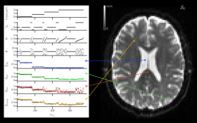
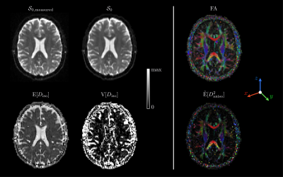
Statistical descriptors of interest: The mean diffusivity

$\mathrm{E}[D_\mathrm{iso}]$ , variance of isotropic diffusivities

$\mathrm{V}[D_\mathrm{iso}]$ , and normalized mean anisotropy

$\tilde{\mathrm{E}}[D_\mathrm{aniso}^2]=\mathrm{E}[(D_\mathrm{iso}D_\Delta)^2]/\mathrm{E}[D_\mathrm{iso}]^2$ (similar to the microscopic

$\mathrm{FA}$ ),¹⁰ with the isotropic diffusivity

$D_\mathrm{iso}$ , normalized diffusion anisotropy

$D_\Delta\in[-0.5,1]$ , and the voxel-scale expectation and variance

$\mathrm{E}[\cdot]$ and

$\mathrm{V}[\cdot]$ , respectively.

In vivo human brain: After implementing an iterative fitting of

$\mathcal{S}_\Gamma$ in Matlab,²⁰ we applied it to a dataset available online,²¹ which signal-to-noise ratio (SNR) was around 30 in the corona radiata.²² Fig.1 presents the acquisition scheme and shows that mv-Gamma reasonably fits the signals arising from diverse voxel contents. Fig.2 features consistent estimated parameter maps of

$\mathcal{S}_0$ ,

$\mathrm{E}[D_\mathrm{iso}]$ ,

$\mathrm{V}[D_\mathrm{iso}]$ and

$\mathrm{FA}$ . However,

$\tilde{\mathrm{E}}[D_\mathrm{aniso}^2]$ vanishes in areas of crossing fibers.

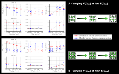
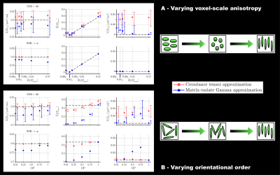
In silico: Various voxel contents were simulated in terms of distributions of

$D_\mathrm{iso}$ ,

$D_\Delta$ and orientations, with identical in vivo acquisition scheme and SNR. Medians and interquartile ranges on estimating

$\mathrm{E}[D_\mathrm{iso}]$ ,

$\tilde{\mathrm{E}}[D_\mathrm{aniso}^2]$ and

$\mathrm{V}[D_\mathrm{iso}]$ were assessed across 100 Rician-noise realizations of the covariance tensor approximation (Cov)¹¹ and the matrix-variate Gamma approximation (MV-Gamma), and compared to the simulated ground truth in isotropic (Fig.3) and anisotropic (Fig.4) systems. MV-Gamma adequately captures voxel-scale anisotropy and shows superior performance to Cov in accurately capturing

$\mathrm{V}[D_\mathrm{iso}]$ , but is inferior in estimating

$\mathrm{E}[D_\mathrm{iso}]$ . Besides, it cannot capture sub-voxel anisotropy (

$\tilde{\mathrm{E}}[D_\mathrm{aniso}^2]$ ) in anisotropic systems with low orientational order, thereby confirming the previous in vivo observations.

Conclusion

We defined matrix moments enabling the computation of diffusion metrics for any functional choice approximating a diffusion tensor distribution

$\mathcal{P}(\mathbf{D})$ . Applying these tools to the mv-Gamma distribution up to its second matrix moment yields a new signal representation, the matrix-variate Gamma approximation, that performs adequately in orientationally ordered anisotropic systems (further justifying its use within DIAMOND),^14,15 but misses sub-voxel anisotropy in systems with low orientational order. This missing information is likely contained in the sixth-order skewness tensor, which can be obtained via a third matrix moment.

Acknowledgements

This work was financially supported by the Swedish Foundation for Strategic Research (AM13-0090, ITM17-0267) and the Swedish Research Council (2018-03697).

References

1. Jian B et al., A novel tensor distribution model for the diffusion-weighted MR signal. Neuroimage 2007;37(1):164-176

2. Eriksson S et al., Isotropic diffusion weighting in PGSE NMR by magic-angle spinning of the q-vector. Journal of Magnetic Resonance 2013;226:13-18.

3. Eriksson S et al., NMR diffusion-encoding with axial symmetry and variable anisotropy: Distinguishing between prolate and oblate microscopic diffusion tensors with unknown orientation distribution. The Journal of Chemical Physics 2015;142(10):104201.

4. Topgaard D, Multidimensional diffusion MRI. Journal of Magnetic Resonance 2017; 275:98-113.

5. de Almeida Martins J P and Topgaard D, Two-dimensional correlation of isotropic and directional diffusion using NMR. Physics Review Letters 2016;116:087601.

6. de Almeida Martins J P and Topgaard, D Multidimensional correlation of nuclear relaxation rates and diffusion tensors for model-free investigations of heterogeneous anisotropic porous materials. Scientific Reports 2018;8,2488.

7. Topgaard D. Diffusion tensor distribution imaging. NMR in Biomedicine 2019;32(5):e4066

8. Yablonskiy D A et al., Statistical model for diffusion attenuated MR signal, Magnetic Resonance in Medicine 2003;50:664.

9. Jbabdi S et al., Model-based analysis of multishell diffusion MR data for tractography: How to get over fitting problems. Magnetic Resonance in Medicine 2012;68:1846.

10. Lasic S et al., Microanisotropy imaging: quantification of microscopic diffusion anisotropy and orientational order parameter by diffusion MRI with magic-angle spinning of the q-vector. Frontiers in Physics 2014;2:11.

11. Westin C-F et al. Q-space trajectory imaging for multidimensional diffusion MRI of the human brain. NeuroImage 2016;135:345-362.

12. Guptar A K and Nagar D K, Matrix Variate Distributions. Edited by Chapman and Hall/CRC, Boca Raton, Florida, 2000.

13. Scherrer B et al., Characterizing brain tissue by assessment of the distribution of anisotropic microstructural environments in diffusion-compartment imaging (DIAMOND). Magnetic Resonance in Medicine 2016;76:963.

14. Scherrer B et al., Decoupling axial and radial tissue heterogeneity in diffusion compartment imaging. In: Information Processing in Medical Imaging (IPMI) 2017;440-452.

15. Reymbaut A et al., The “Magic DIAMOND" method: probing brain microstructure by combining b-tensor encoding and advanced diffusion compartment imaging. In: International Society for Magnetic Resonance Imaging (ISMRM) 2018.

16. Brewer J, Kronecker products and matrix calculus in system theory. IEEE Transactions on Circuits and Systems 1978;25:772.

17. Laue S et al., Computing higher order derivatives of matrix and tensor expressions. In: Advances in Neural Information Processing Systems (NIPS) 2018.

18. Laue S et al., Matrix calculus, www.matrixcalculus.org. Accessed: 2019-07-30.

19. Higham N J, Computing a nearest symmetric positive semidefinite matrix. Linear algebra and its applications 1988;103:103-118.

20. Nilsson M et al., An open-source framework for analysis of multidimensional diffusion MRI data implemented in MATLAB. In: International Society for Magnetic Resonance Imaging (ISMRM) 2018.

21. Szczepankiewicz F et al., Linear, planar and spherical tensor-valued diffusion MRI data by free waveform encoding in healthy brain, water, oil and liquid crystals. Data in Brief 2019;25:104208.

22. Szczepankiewicz F et al., Tensor-valued diffusion encoding for diffusional variance decomposition (DIVIDE): Technical feasibility in clinical MRI systems. PLoS ONE 2019;14(3):e0214238.

Figures

Figure 1. Left: Acquisition scheme (

$\mathbf{b}$ 's trace

$b$ , normalized anisotropy

$b_\Delta$ and orientation

$(\Theta,\Phi)$ ) with sorted acquisition number

$n_\mathrm{acq}$ , and measured (black) and fitted (color) normalized signals

$\tilde{S}$ in selected voxels (cerebrospinal fluid in blue, grey matter in green, white matter in red, and crossing area in orange). Right:

$\mathcal{S}_0$ map indicating the location of the selected voxels.

Figure 2. Left: Estimated axial parameter maps of

$\mathcal{S}_0$ (compared to the measured

$\mathcal{S}_{0,\mathrm{measured}}$ ),

$\mathrm{E}[D_\mathrm{iso}]$ and

$\mathrm{V}[D_\mathrm{iso}]$ . Grey scale codes for magnitude. Right: Estimated axial parameter maps of

$\mathrm{FA}$ and

$\tilde{E}[D_\mathrm{aniso}^2]$ . Color codes for orientations and opacity codes for magnitude.

Figure 3. Characterization of isotropic systems with varying

$\mathrm{V}[D_\mathrm{iso}]$ at low

$\mathrm{E}[D_\mathrm{iso}]$ (top), and at high

$\mathrm{E}[D_\mathrm{iso}]$ (bottom). Each system consists of two identical Gaussian distributions of

$D_\mathrm{iso}$ . While the left panels feature both SNR=30 and infinite-SNR results, the right panels illustrate the voxel contents for both cases.

Figure 4. Characterization of anisotropic components with constant orientation and varying

$\tilde{E}[D_\mathrm{aniso}^2]$ (top), and with varying orientational order and constant

$\tilde{E}[D_\mathrm{aniso}^2]$ (bottom). The order parameter

$\mathrm{OP}=\mathrm{E}[P_2(\cos\theta)]$ (with second Legendre polynomial

$P_2$ ) is set by a Watson distribution of these identical components (Gaussian distributions of

$D_\Delta$ with constant

$\mathrm{E}[D_\mathrm{iso}]$ ). Other conventions are identical to those of Figure 3.

Proc. Intl. Soc. Mag. Reson. Med. 28 (2020)

4408