Introduction

Employing optimal designs criteria¹, such as the minimization of parameter variances through the Cramer-Rao Lower Bound, is a known practice in the field of diffusion MRI^2,3. Nevertheless, it can be computationally tedious to search the entirety of the independent variables space, with the risk of ending with a supposedly optimal setting without the general picture of how the employed model effectively reacts to different experimental conditions. Generalized sensitivity functions⁴ (GSFs) are studied in biological models to visually assess which temporal observations are most informative for single parameters: in the present study we reformulate their concept to understand which b-value ranges play a central role for accurate model identification in the diffusion MRI field.

Methods

The generalized sensitivity analysis we propose evaluates the Fisher Information associated with a diffusion shell at specific b-values and normalizes it by the summation of the Fisher information over an entire b-value range. We define the Generalized Sensitivity matrix as:

$$ \mathbf{GS}(b_{J})=\sum_{j=1}^{J}{\left[\sum_{m=1}^{M}{\mathbf{I_\theta}}{(b_{m})}\right]^{-1} \mathbf{I_\theta}}({b_{j})}\hphantom{aaaaaaah}[1] $$

where $$$ \mathbf{GS} $$$ is the Generalized Sensitivity matrix, $$$ M $$$ is the length of the b-value vector $$$\mathbf{b}=[b_{1},b_{2},...,b_{M}] $$$, and $$$ \mathbf{I_\theta} $$$ is the shell-wise Fisher Information matrix, whose exact formulation depends on the biophysical model and the noise probability density function. For the most common Gaussian case, $$$ \mathbf{I_\theta} $$$ becomes⁵:
$$ (\mathbf{I_{\theta}})_{i,j}(b)=\sum_{\mathbf{g}\in\mathbf{G}}{\frac{1}{\sigma^{2}(b)}}\mathbf{\nabla}_{\theta}[\tilde{S}(b,\mathbf{g},\theta_{i})]\mathbf{\nabla}_{\theta}[\tilde{S}(b,\mathbf{g},\theta_{i})]\hphantom{aaaaaaah}[2] $$
where $$$\mathbf{G}$$$ is the set containing all the diffusion gradient directions, $$$ \nabla_{\theta} $$$ denotes the gradient operator with respect to the model parameters and $$$\tilde{S}$$$ is the studied biophysical model prediction. The generalized sensitivity functions for the model parameters are then extracted from the GS matrix in [1]:
$$ \mathbf{gsf_{\theta}}(b_{J}) =diag(\mathbf{GS}(b_{J}))\hphantom{aaaaaaah}[3] $$
As GSFs are cumulative functions, the most informative shells are associated with the steepest increase of their trajectories⁴.

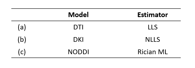
We demonstrate the usefulness of GSFs by providing their visualization for the DTI⁶ and DKI⁷ signal representations, as well as for the Neurite Orientation Dispersion and Density Imaging⁸ (NODDI) biophysical model. GSFs require a parameter vector $$$\mathbf{\theta}_{0}$$$ containing the model parameters for their generation. We identify such vector by fitting each model on a healthy subject from the publicly available data of the Human Connectome Project⁹ (b1/b2=1000/3000 s/mm², 64 directions each) and taking the estimates from one representative voxel in the Corpus Callosum. We investigate diffusion shells in the range b∈[0-5000] s/mm² with a fixed number of 30 isotropically dispersed gradient directions each. Table 1 shows the different estimators according to which GSFs were generated.

Results&Discussion

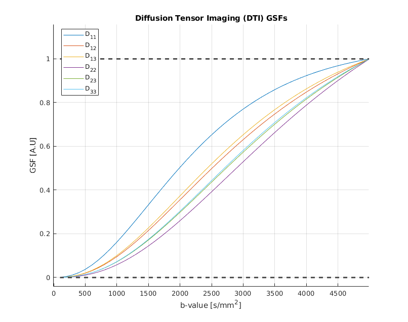
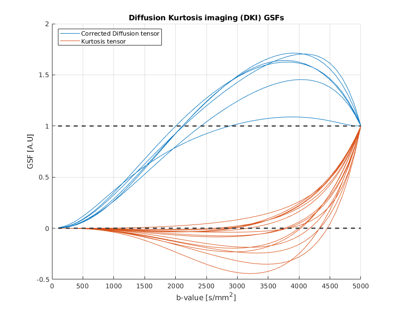
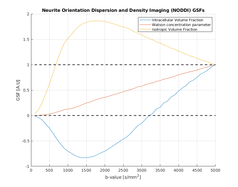
Figure 1 shows the GSFs for the six independent parameters of the classic diffusion tensor. It is important to note that each parameter trajectory has unitary value at the end of the studied b-value interval: this a structural consequence which can be explained by evaluating [1] when J=M. Failure to “sum up to one” is usually caused by badly conditioned Fisher matrices. While the single tensorial components have slightly different curves, their general behaviour is the same, exhibiting the steepest increase (and thus, the most information gain) in the interval [1000-2500] s/mm², value for which the curves are starting to plateau. DKI parameters sensitivity curves are shown in Figure 2. It is straightforward to detect two different patterns in this case. The first one is similar to the GSFs in Figure 1, and it is followed by the six parameters representing the kurtosis-corrected diffusion tensor, with an optimal range of b-values around 1000-1500 s/mm² ; the second one belongs to the Kurtosis Tensor components, for which the information gain starts from b=2500 s/mm² onwards. Thus, the present method effectively suggests the necessity of two b-shells in order to accurately estimate all DKI parameters. Figure 2 also features significant under/overshoots from the [0-1] range: these issues are present when the non-diagonal elements of are significantly large, which in turn are caused by large correlations amongst different parameters⁵. It is interesting how the kurtosis-corrected diffusion tensor GSFs rise earlier than their classic DTI counterparts. Figure 3 introduces NODDI sensitivities for the three scalar parameters. The GSFs of the two volume fractions present large overshoots/undershoots, thus exposing the high structural correlation which links them. The isotropic volume estimation highly benefits from a shell in the 200-900 s/mm² range, while the intracellular volume features a pronounced information gain with a shell from b=1500 s/mm² onwards: these findings agree with the proposed optimized NODDI protocol⁸. Interestingly, we find the Watson concentration parameter (conveying the information of the Orientation Dispersion Index) has no optimal ranges for its estimation and draws its precision equally across the studied b-value space.

Conclusions

The present work introduces generalized sensitivity functions as a strategy for visually exploring which ranges of b-value are most informative for model parameters when defining HARDI acquisition protocols. Amongst the results, we were able to expose two distinct optimal intervals for the DKI tensors and the NODDI volumetric fractions, along with the poor sensitivity of the Watson concentration parameter, in accordance with literature. GSFs are not meant to substitute optimal experiment design procedures, but can rather provide characterizing information for proper contextualization of their results; they are computationally light to generate and employ information easily derivable by standard fitting routines, supporting their inclusion in standard modeling analyses.

Acknowledgements

No acknowledgement found.