4394
A simple phantom for extracting Intravoxel Incoherent Motion (IVIM) model parameters1Physics, Texas Center for Superconductivity at University of Houston, Houston, TX, United States, 2Diagnostic and Interventional Radiology, Baylor St. Luke's Medical Center, Houston, TX, United States
Synopsis
We present a simple phantom set-up to model diffusion weighted imaging signal arising from intra-voxel incoherent motion (IVIM). The model provides means to independently control both the perfusion fraction (f) as well as the pseudodiffusion coefficient (Df).
Synopsis
We present a simple phantom set-up to model diffusion weighted imaging signal arising from intra-voxel incoherent motion (IVIM). The model provides means to independently control both the perfusion fraction (f) as well as the pseudodiffusion coefficient (Df). Across a range of flow velocities, numerical simulations and phantom experiments confirm that: (a) perfusion fraction (f) is overestimated by traditional analysis approaches such as segmented (S), or oversegmented (OS) methods, but is slightly underestimated by the AS-T2 method; (b) Df increases in proportion to flow velocity, and the estimation of Df is unaffected by the analysis technique.Introduction
Since the initial description of IVIM phenomena by LeBihan1, several groups have suggested various approaches to create phantom models to simulate physiologic conditions 2-4. This has been a challenging issue as tissue diffusion (Dt) and fluid diffusion (Df) vary by two orders of magnitude or more, and creation of physical models with well-defined perfusion volume fractions (f) is also difficult. In this work, we present a simple phantom model that can be used to synthesize signals mimicking IVIM phenomena which can be used to evaluate the performance of various analysis algorithms in the estimation of parameters such as f, and Df.METHODS
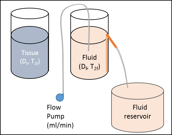
IVIM Phantom: A cartoon representation of the phantom model used to generate IVIM signal is shown in Figure 1. A small cylinder of known diameter filled with material of desired diffusivity, and desired T2 relaxation time serves as a representation of static tissue (Dt, and T2t), and fluid with desired T2 (T2f) is pumped into another cylindrical container with a spout at a specific height which is connected to a straw with an opening at the bottom of the container, acts as a representation of fluid compartment. The same fluid is pumped into the fluid compartment using a peristaltic pump at a constant flow rate, and a steady state is established when the inflow rate equals the outflow rate at the spout which flows into the reservoir of the pump. Adjusting the flow rate alters the fluid velocity (V) within the fluid compartment, thereby altering Df.Signal generation: This phantom set up can now be imaged using diffusion weighted imaging with various ‘b’ values, with the static tissue compartment and the fluid compartment within the imaging field of view, and when the flow across the fluid compartment is in steady state.
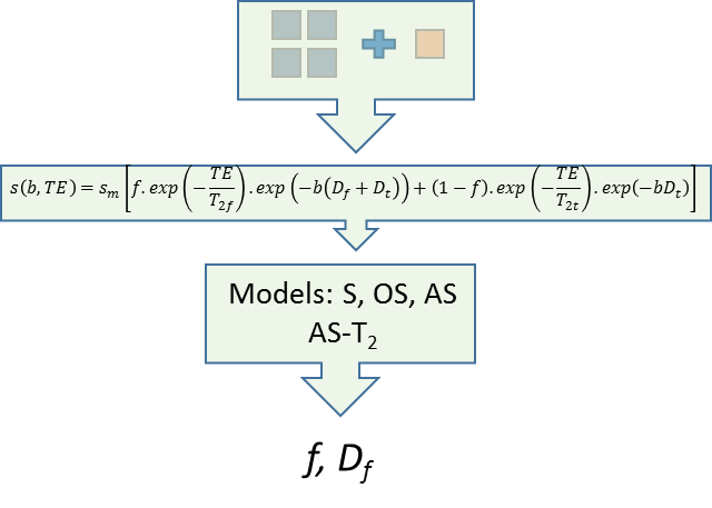
Controlling perfusion fraction (f) :Now depending on the perfusion fraction desired, the ratio of pixels from the static and fluid compartments can be randomly picked, e.g., if a perfusion fraction of 20% is desired, the ratio of pixels chosen from the static tissue compartment and flowing compartment will be 4:1. The addition of these measured signals will yield an IVIM signal curve that includes the effect of the diffusivities and relaxation rate differences between the two compartments (Figure 2).
Controlling pseudo-diffusion coefficient (Df ): To attain a pre-determined value of Df without the confounding effects of relaxation rate differences, the diffusion weighted signal just from the flowing compartment is fitted with the biexponential IVIM model to extract the value of Df as a function of flow velocity which can be estimated from the input flow rate from the peristaltic pump and the geometry of the fluid compartment (cylinder, in this instance).
Numerical Simulations: MR signal was simulated using Eq. 1 with Df as in Eq. 6. The following were fixed to mimic our phantom: f 0.25, Dt 0.002 mm2/s, l 0.7354 mm, T2f 97.3 ms, T2t 63.5 ms, 10 b values (0,10,25,50,75,100,200,300,500,800 s/mm2). We also varied V from 0 to 0.921 mm/s and 8 TE ranging from 0 to 150 ms. Gaussian noise was added to generate MR signal for each sample at SNR levels of 20 and 50. Each sample was simulated 5000 times.
Phantom: Two phantoms with different T2 values, 63.5 ms and 97.3 ms were made using water doped with Gd to represent tissue and fluid compartments respectively. Fluid compartment was passed through a bottle of diameter 48 mm at 5 different flow rates (0, 40, 60, 80, 100 mL/min) resulting into velocities ranging from 0 to 0.921 mm/s.
MR acquisition : Diffusion Weighted Imaging (DWI) signals were acquired from a 1.5 T scanner using the following parameters: FOV 319 mm X 165 mm , Voxel size 3 mm X 3 mm X 10 mm, TR 2000ms, TE 60 ms and 10 b values as used in the simulation.
RESULTS
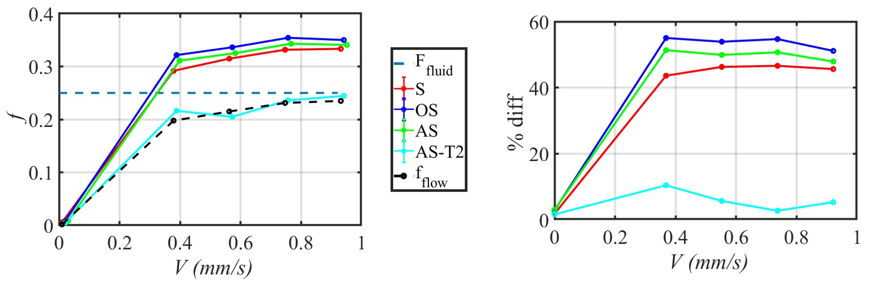
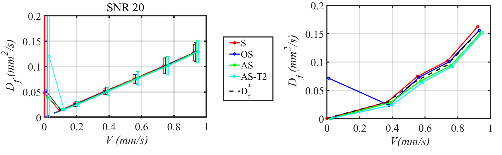
(1) Numerical simulations show that IVIM analysis methods (S, OS, AS) which do not address the T2 differences between the tissue and fluid compartments overestimate f by as much as 40% at a fixed TE of 60 ms, but with T2 correction, correct value of f can be obtained at all fluid velocities (Figure 3). These numerical simulations are verified from the experimental measurements at various flow velocities (Figure 4). (2) The estimated Df as a function of V for simulated and measured signals is shown in Figure 5.CONCLUSION
The proposed phantom model is flexible to generate arbitrary signals with different combinations of f and Df, and is easy to include the effect of tissue relaxation rate differences between the compartments.Acknowledgements
No acknowledgement found.References
1. Le Bihan, D., Breton, E., Lallemand, D., Aubin, M. L., Vignaud, J., & Laval-Jeantet, M. (1988). Separation of diffusion and perfusion in intravoxel incoherent motion MR imaging. Radiology, 168(2), 497-505.
2. Schneider, M., Gaaß, T., Dinkel, J., Ingrisch, M., Reiser, M., & Dietrich, O. (2016). Intravoxel incoherent motion MRI in a 3‐dimensional microvascular flow phantom. In Proc Int Soc Magn Reson Med (Vol. 24, p. 0920).
3. Cho, G. Y., Kim, S., Jensen, J. H., Storey, P., Sodickson, D. K., & Sigmund, E. E. (2012). A versatile flow phantom for intravoxel incoherent motion MRI. Magnetic resonance in medicine, 67(6), 1710-1720.
4. Lorenz, C. H., Pickens III, D. R., Puffer, D. B., & Price, R. R. (1991). Magnetic resonance diffusion/perfusion phantom experiments. Magnetic resonance in medicine, 19(2), 254-260.
Figures