INTRODUCTION

Quasi-Diffusion Magnetic Resonance Imaging (QDI) is a new ultra-high b-value diffusion magnetic resonance imaging (dMRI) technique based on a special case of the Continuous Time Random Walk (CTRW) model of diffusion dynamics^1,2 which assumes the presence of non-Gaussian diffusion properties within tissue microstructure. The QDI technique parameterises the diffusion signal attenuation according to the rate of decay D_1,2 (i.e. the diffusion coefficient in mm²s^-1) and the shape of the power law tail, $$$\alpha$$$. In particular, QDI provides conventional dMRI contrast, and $$$\alpha$$$ maps which are analogous to the Diffusional Kurtosis Imaging (DKI) $$$\kappa$$$ measure³. A minimal tensor QDI acquisition requires a b=0 s mm^-2 image followed by 2 non-zero b-value images in 6 diffusion gradient directions. Here we optimise this minimal QDTI acquisition with respect to a ‘gold standard’ to enable rapid acquisition of high tissue contrast QDI data within a clinically feasible acquisition time of approximately 2 minutes.

METHODS

MRI acquisition
Whole-brain axial dMRI were acquired on a 3T Philips Dual Achieva TX system using a single-shot diffusion sensitised EPI sequence (TE=90ms, TR=6000ms, 1.5mm×1.5mm×5mm) in 6 non-collinear diffusion gradient directions for 5 healthy individuals (age 22±4.5 years). The ‘gold standard’ involved acquisition of 28 diffusion-sensitised images at equally spaced intervals from b = 180 to 5000 s mm^-2 ($$$\delta$$$=23.5ms, $$$\Delta$$$=43.9ms) and 10 b=0 s mm^-2 images. Images were acquired twice to increase signal-to-noise in a total time of 35minutes 36seconds.

Image analysis
Permutation analysis was performed for each pair of non-zero b-values taken from the gold standard acquisition (n=387 permutations). The QDI model was fitted for the gold standard and each b-value pair at each voxel to the following equation for signal, S, in each diffusion gradient direction,
$$
S_{b}=S_{0}\sum_{k=0}^{\infty}\frac{(-1)^{k}(D_{1,2}b)^{\alpha k}}{\Gamma(\alpha k+1)}, [Eq.1]
$$
Model fitting was performed on denoised⁴ dMRI data using the Levenberg-Marquadt algorithm and Padé approximation to rapidly estimate Eq.1 and its derivatives⁵. The $$$\chi^2$$$ difference between the diffusion signal decay curves for the gold-standard and each b-value permutation (across 28 b-values between 0 and 5000 s mm^-2) were calculated at each voxel and averaged across diffusion gradient directions. Grey and white matter voxels were identified at 95% tissue probability from T1-weighted images⁶ (1mm³ voxel resolution) that were aligned⁷ to the QDI data. Optimisation was performed by minimising the median $$$\chi^2$$$ value of grey and white matter voxels. Tensor maps of D_1,2 and $$$\alpha$$$ were computed⁸ for the optimised and gold standard acquisitions from which mean and anisotropy maps were calculated. Measurement accuracy for mean and anisotropy D_1,2 and $$$\alpha$$$ parameters was investigated in grey and white matter using Bland-Altman plots and paired t-tests between the optimised and gold standard acquisition.

RESULTS

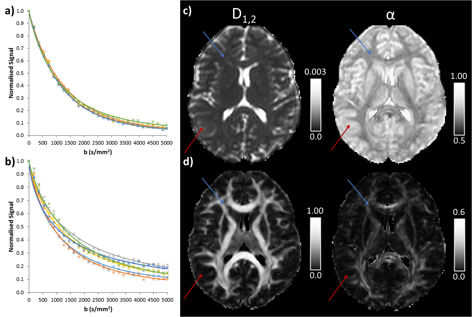
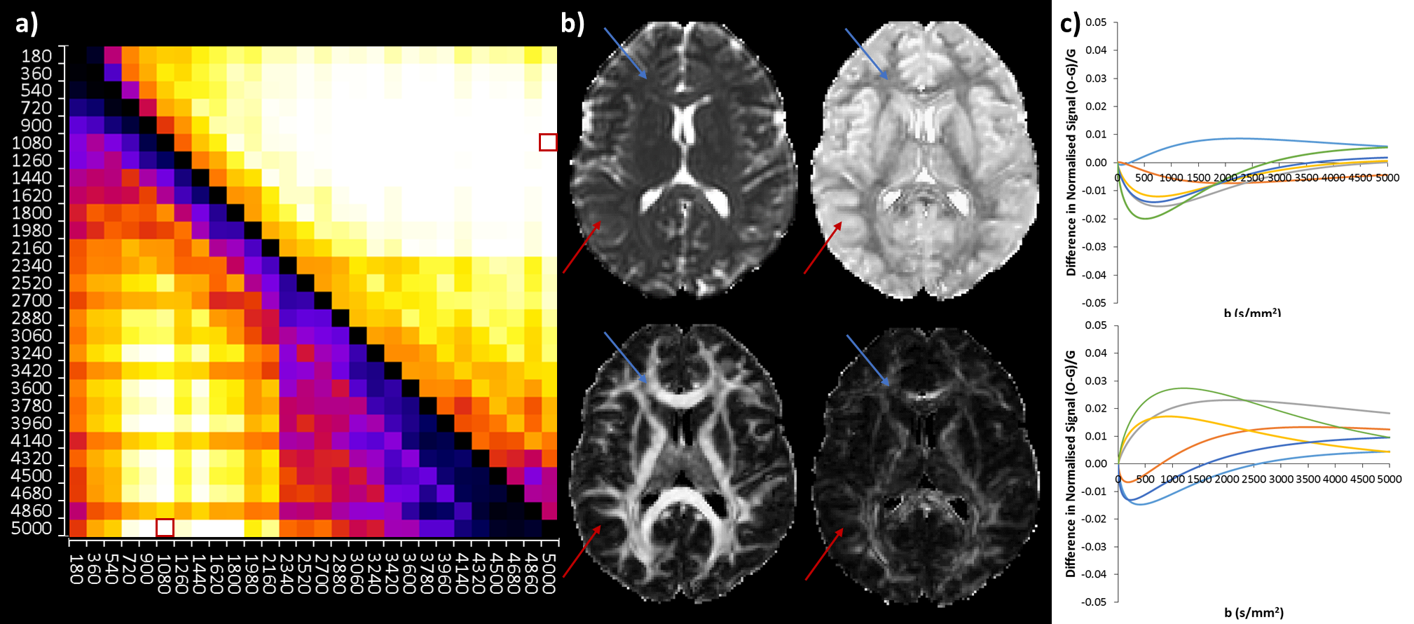
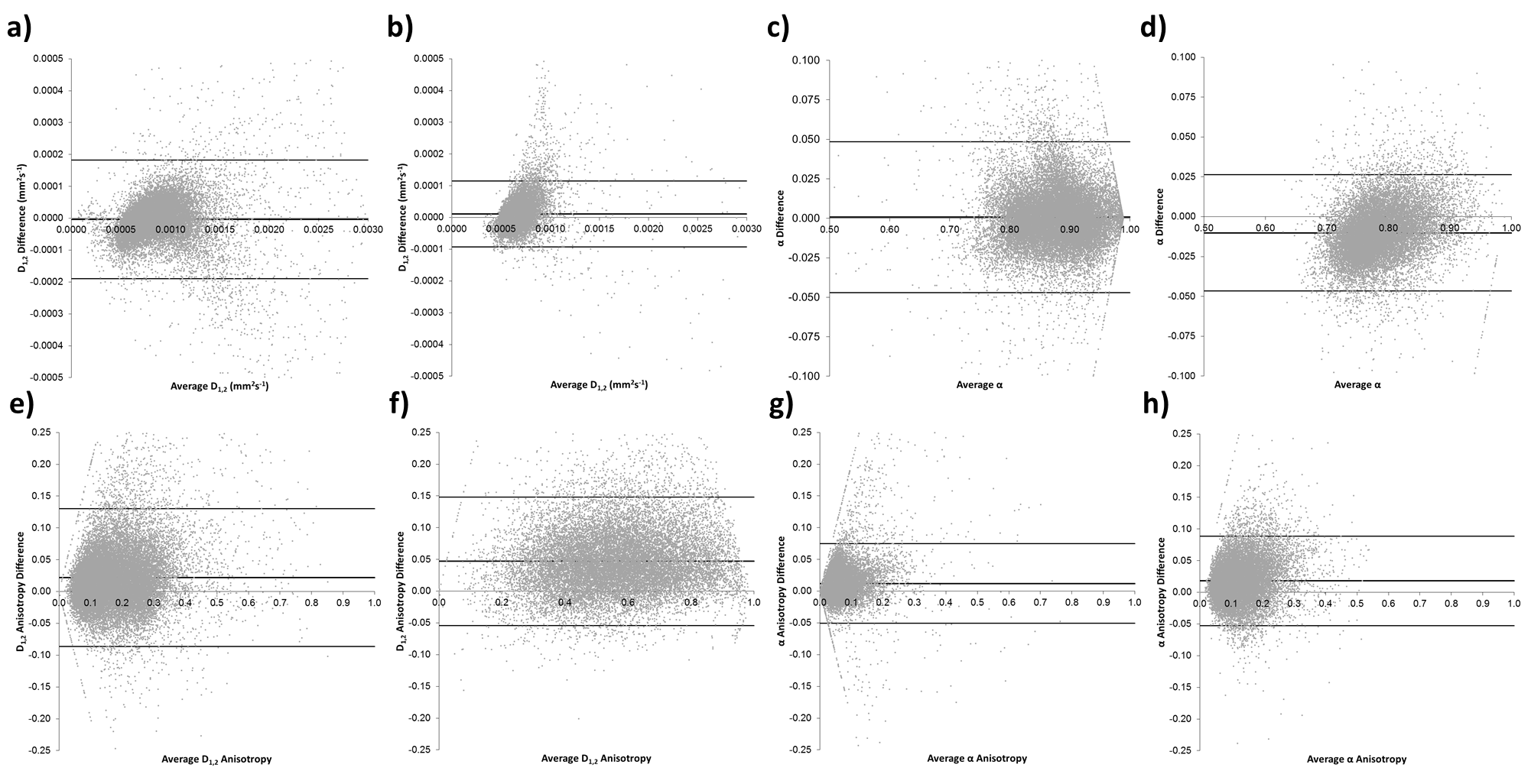
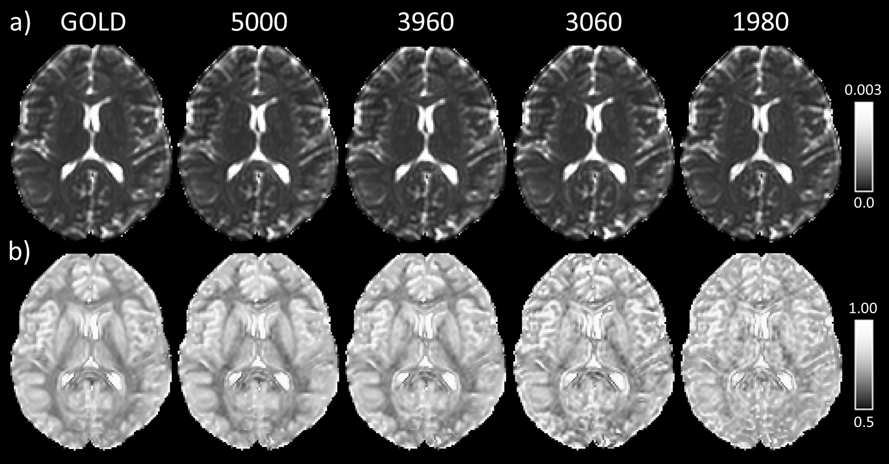
Figure 1 shows gold standard QDI model fits to representative grey and white matter voxels and gold standard maps of D_1,2 and $$$\alpha$$$ maps. The gold standard maps exhibit excellent tissue contrast.

The optimisation results are shown in Figure 2a and indicate that the diffusion signal decay curve for the b=0, 1080, 5000 s mm^-2 combination most closely matches the gold standard decay curve ($$$\chi^2$$$ = 0.030±0.007). Optimised parameter maps provide excellent tissue contrast (Figure 2b) and are visually similar to the gold standard data (Figure 1). Graphs of the difference between signal decay curves for the gold standard and optimal b-value combination for the representative grey and white matter voxels (Figure 2c) show a maximum deviation from the gold standard of 2.00% in grey and 2.73% in white matter. Bland-Altman plots (Figure 3) indicate that the optimal b-value combination overestimates mean D_1,2 (average difference = 0.016±0.011 x10^-3 mm²s^-1) and underestimates mean $$$\alpha$$$ (average difference = -0.014±0.004) in white matter. D_1,2 and $$$\alpha$$$ anisotropy were also overestimated in grey (average difference = 0.019±0.004 and 0.013±0.002, respectively) and white matter (average difference = 0.043±0.011 and 0.018±0.003, respectively). Paired t-tests indicate that the small differences between the optimal and gold standard QDI parameters are significant (p<0.05) for mean D_1,2 and $$$\alpha$$$ and in white matter and D_1,2 and $$$\alpha$$$ anisotropy in grey and white matter. Figures 4 & 5 shows mean and anisotropy QDI maps for optimised b-value pairs with maximum b-values (b_max) of approximately 4000, 3000 and 2000 s mm^-2 compared to the gold standard and optimal data. Tissue contrast visibly deteriorates with reduction of maximum b-value as indicated by increases in $$$\chi^2$$$ ($$$\chi^2$$$ = 0.034±0.011; 0.054±0.017; 0.127±0.032, respectively).

DISCUSSION AND CONCLUSION

We have identified an optimal QDI acquisition that provides a short clinically feasible protocol with excellent tissue contrast. The acquisition time of our optimal QDTI is 3 minutes 24 seconds. As we acquired data twice to increase signal to noise ratio, a shorter optimal acquisition could be acquired in approximately 2 minutes (i.e. 132 seconds), albeit with a loss in signal to noise ratio. This could be further shortened to 96 seconds for a 3 orthogonal diffusion direction acquisition. Our optimised acquisitions with lower maximum b-values could be acquired on systems that have diffusion gradient limitations to provide good tissue contrast for b_max≥4000 s mm^-2 or calculated from existing dMRI datasets. The short acquisition time identified by our optimal QDTI protocol indicates that QDI may be added to routine conventional dMRI acquisition allowing simple translation to the clinical arena.

Acknowledgements

Funding for this study was provided by a St George’s, University of London Innovation Award.