4371

Automated feature extraction across scanners for harmonization of diffusion MRI datasets

Samuel St-Jean¹, Max A. Viergever¹, and Alexander Leemans¹
¹Image sciences institute, University Medical Center Utrecht, Utrecht, Netherlands

Synopsis

Small variations in diffusion MRI metrics between subjects are ubiquitous due to differences in scanner hardware and are entangled in the genuine biological variability between subjects, including abnormality due to disease. In this work, we propose a new harmonization algorithm based on adaptive dictionary learning to mitigate the unwanted variability caused by different scanner hardware while preserving the biological variability of the data. Results show that unpaired datasets from multiple scanners can be mapped to a scanner agnostic space while preserving genuine anatomical variability, reducing scanner effects and preserving simulated edema added to test datasets only.

Introduction

Quantitative scalar measures of diffusion MRI datasets are subject to normal variability across subjects, but potentially abnormal values may yield essential information to support analysis of controls and patients cohorts. However, small changes in the measured signal due to differences in scanner hardware or reconstruction methods in parallel MRI^1,2,3 may translate into small differences in diffusion metrics such as fractional anisotropy (FA) and mean diffusivity (MD)⁴. In the presence of disease, these small variations are entangled in the genuine biological variability between subjects. In this work, we propose a new harmonization algorithm based on adaptive dictionary learning to mitigate the unwanted variability caused by different scanner hardware while preserving the natural biological variability present in the data⁵.

Methods

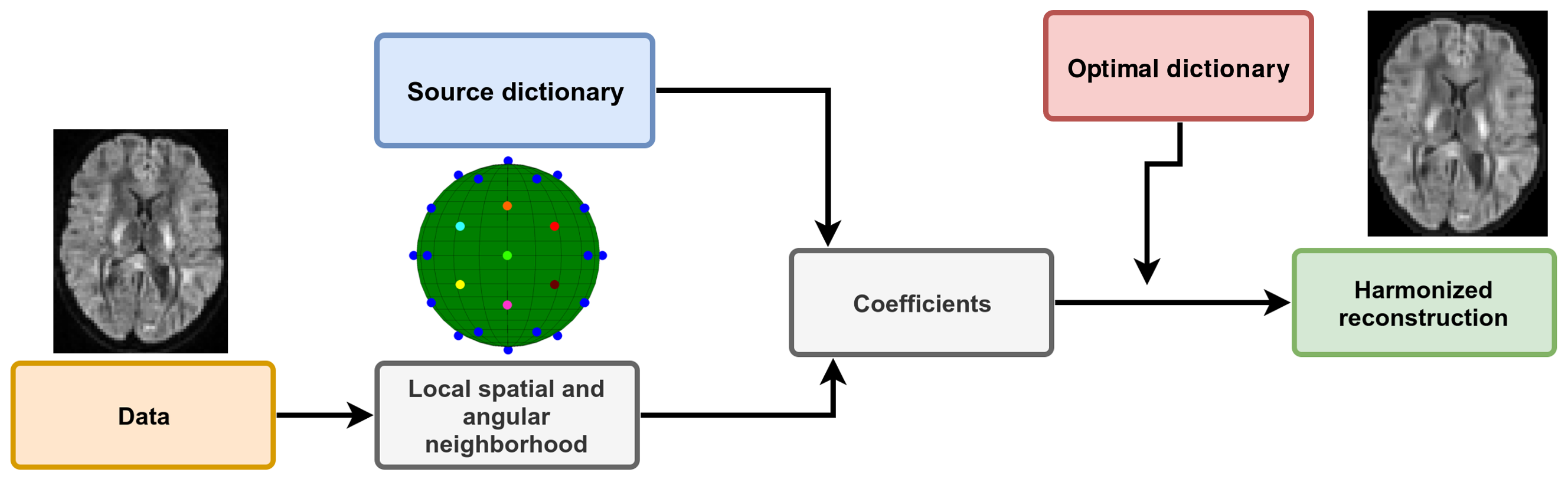
A dictionary is formed from local windows of spatial and angular patches extracted from the diffusion weighted images (DWI), exploiting self-similarity of different DWIs at the same spatial location and close on the sphere^6,7. All extracted patches are stored as vectors $$$X_n$$$ and a subset is randomly chosen to initialize the dictionary D. A sparse vector $$$\alpha$$$ can now be computed such that D is a good approximation to $$$X_n≈D\alpha_n$$$ and D can be subsequently updated to better approximate those vectors. At the next iteration, a new set of candidate vectors $$$X_n$$$ is randomly drawn and D is updated to better approximate this new set of vectors. This iterative process can be written as

$$\text{argmin}_{D,\alpha}\frac{1}{N}\sum_{n=1}^N\frac{1}{2}||X_n-D\alpha_n||_2^2+\lambda_i||\alpha_n||_1~\text{s.t.}~||D_{.p}||_2^2=1$$

with $$$\alpha_n$$$ the sparse coefficients, D the dictionary where each column is constrained to unit $$$\ell_2$$$-norm to prevent degenerated solutions and $$$\lambda_i$$$ is an adaptive regularization parameter for iteration $$$i$$$ which is automatically determined⁸ for each individual $$$X_n$$$. This is done with 3-fold cross-validation (CV) and minimizing the mean squared error or by minimizing the Akaike information criterion (AIC)⁹. Once the dictionary has been optimized with patches from all scanners, it should only contain features that are common to all datasets. Approximation with this optimal dictionary therefore discards scanner specific effects from the data as they are not contained in the dictionary itself as detailed in Figure 1.

Datasets

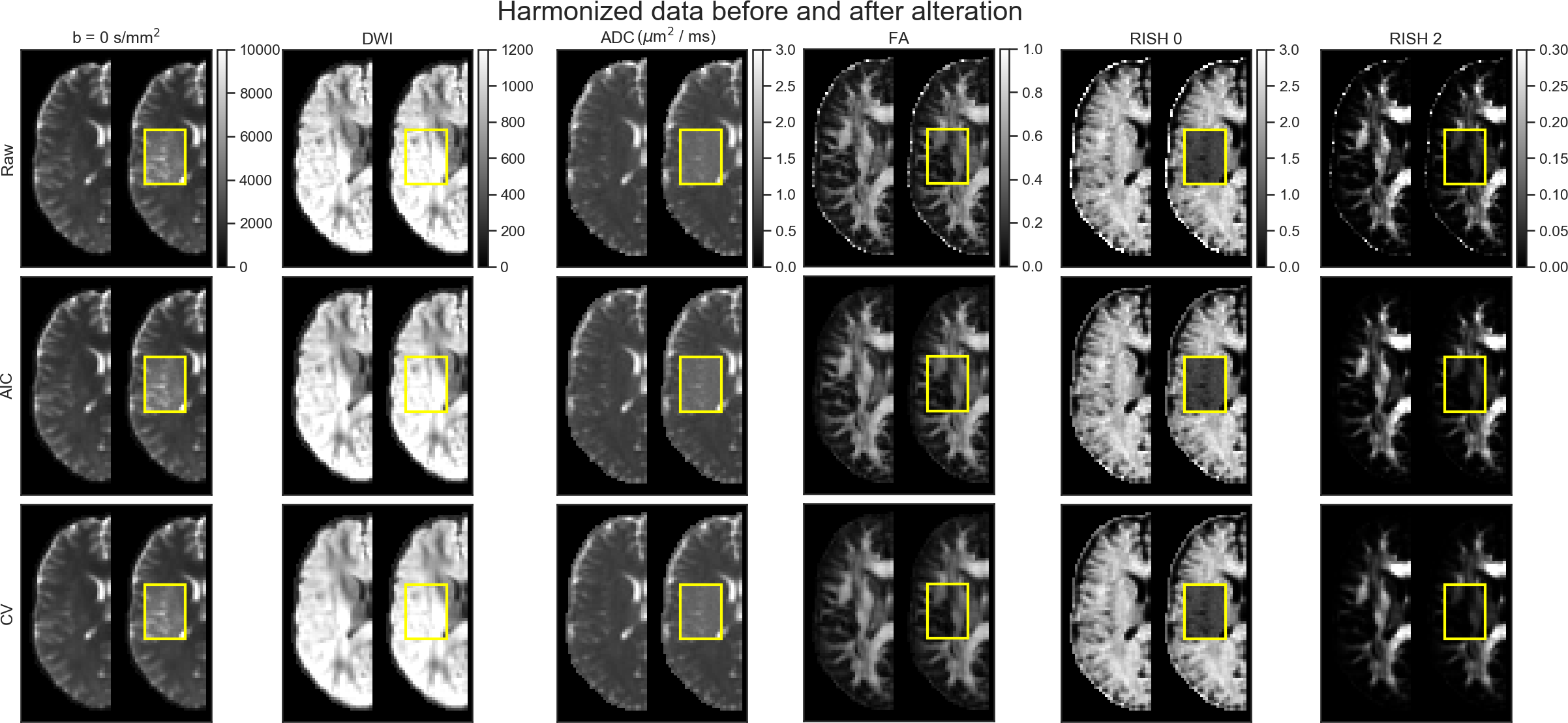
We use the benchmark database from the CDMRI 2017 challenge¹⁰, which consists of ten training subjects and four test subjects acquired on three different scanners (GE with gradient strength of 40 mT/m, Prisma with 80 mT/m and Connectom with 300 mT/m). The database consists of 3 b=0 s/mm² images, 30 DWIs acquired at 3 b=1200 s/mm² at a resolution of 2.4 mm isotropic and TE/TR = 98 ms/7200 ms. Note that the GE datasets were acquired with a cardiac gated TR instead. Standard preprocessing includes motion correction, EPI distortions corrections, image registration and brain extraction for each subject across scanners¹⁰. To ensure that the scanner effects are properly removed without affecting genuine biological variability, the test datasets were altered in a small region (3000 voxels) with a simulated free water compartment to mimick edema according to

$$S_{b_\text{altered}}=S_b+fS_0\exp{(-bD_\text{csf})}$$

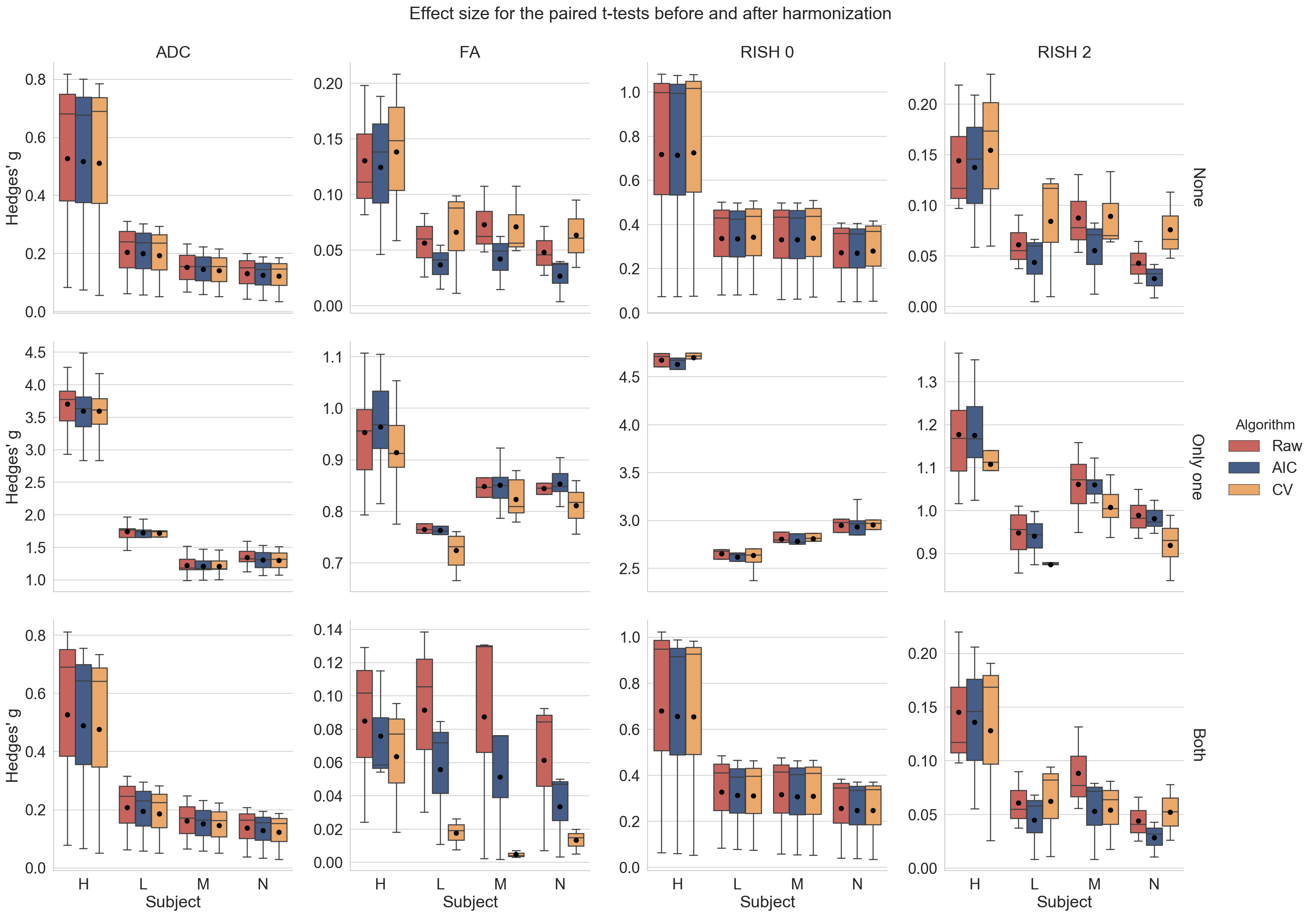
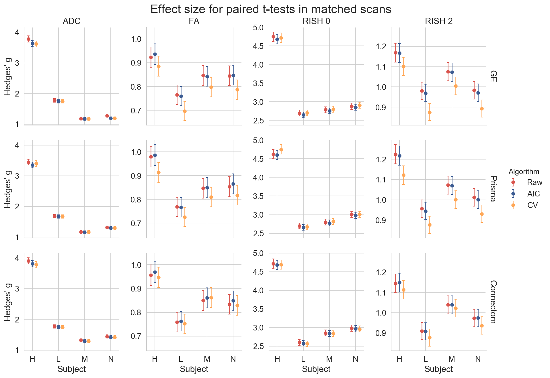
with $$$S_{b_\text{altered}}$$$ the new signal in the voxel, $$$S_b$$$ the original signal in the voxel at b-value b and $$$S_0$$$ the signal in the b=0 s/mm² image, $$$f$$$ is the fraction of the free water compartment¹¹ (drawn randomly for every voxel from a uniform distribution $$$U(0.7,0.9)$$$) and $$$D_\text{csf}=3\times10^{−3}\text{ mm}^2/\text{s}$$$. As these altered datasets are not present in the training set, we can quantify if the induced effects are properly reconstructed. This was done by computing the MD, FA and rotationally invariant spherical harmonics (RISH) features of order 0 and 2 for each dataset as in the original challenge¹⁰. The effect size from a paired t-test was also computed to evaluate if the harmonization algorithm mistakenly removed genuine biological information.

Results

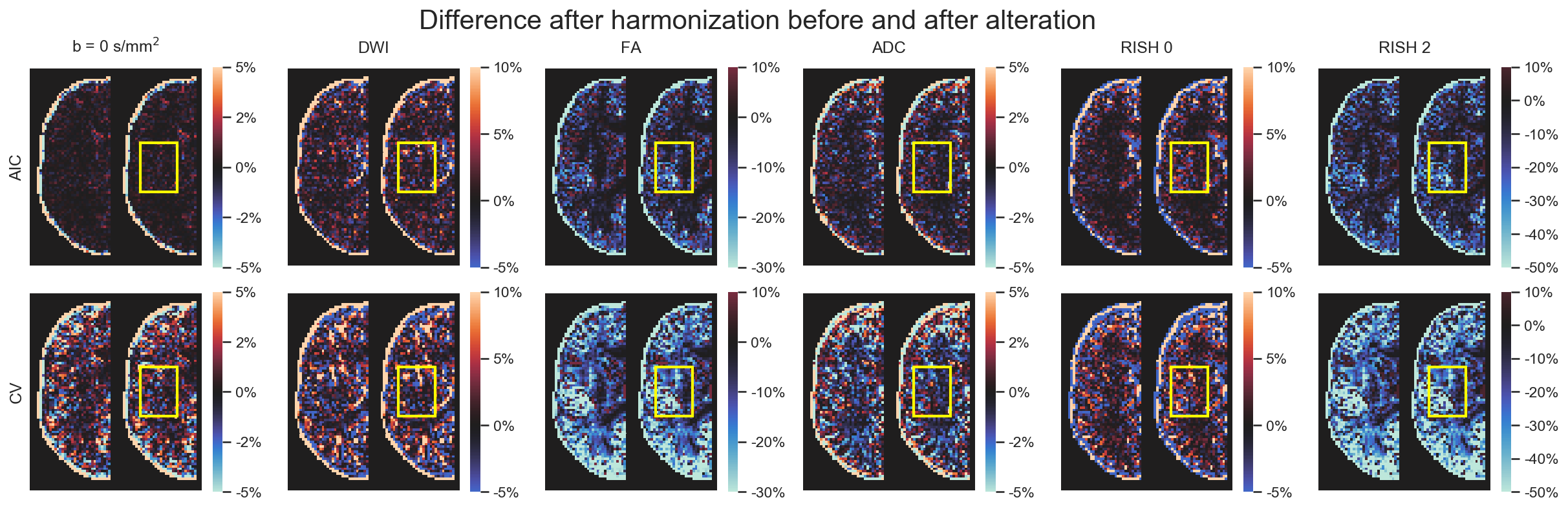
Figure 2 shows the original harmonized data and its metrics (left) and the altered version of those datasets (right) for one subject. The addition of free water changes the metrics, but only slightly affect the DWIs themselves. Figure 3 shows the percentage difference between the non harmonized and harmonized datasets with the AIC and CV based regularization. The CV regularization shows larger difference than the AIC regularization. Figure 4 shows the effect size between the test datasets and their altered version. Harmonization reduces the effect size in general when compared to the raw datasets. Figure 5 shows the 95% confidence interval between the altered and original datasets for the effect size. As most of the confidence intervals are overlapping, this shows that the harmonization procedure does not remove genuine anatomical variability in general.

Discussion and Conclusion

We have shown how a mapping from multiple scanners towards a common space can be constructed automatically through dictionary learning using unpaired training datasets to reduce intra and inter scanner differences. This approach has the benefit of removing variability attributable to multiple scanners, instead of trying to force a source scanner to mimic variability which is solely attributable to a target scanner. Reconstruction of altered versions of the test datasets corrupted by a free water compartment preserved the induced differences, even if such data was not part of the training datasets, while removing variability attributable to scanner effects. The presented algorithm could help multicenter studies in pooling their unpaired datasets while removing scanner specific confounds before computing dMRI scalar metrics.

Acknowledgements

Samuel St-Jean was supported by the Fonds de recherche du Québec - Nature et technologies (FRQNT) (Dossier 192865). This research is supported by VIDI Grant 639.072.411 from the Netherlands Organization for Scientific Research (NWO).

The data were acquired at the UK National Facility for In Vivo MR Imaging of Human Tissue Microstructure located in CUBRIC funded by the EPSRC (grant EP/M029778/1), and The Wolfson Foundation. Acquisition and processing of the data was supported by a Rubicon grant from the NWO (680-50-1527), a Wellcome Trust Investigator Award (096646/Z/11/Z), and a Wellcome Trust Strategic Award (104943/Z/14/Z). This database was initiated by the 2017 and 2018 MICCAI Computational Diffusion MRI committees (Chantal Tax, Francesco Grussu, Enrico Kaden, Lipeng Ning, Jelle Veraart, Elisenda Bonet-Carne, and Farshid Sepehrband) and CUBRIC, Cardiff University (Chantal Tax, Derek Jones, Umesh Rudrapatna, John Evans, Greg Parker, Slawomir Kusmia, Cyril Charron, and David Linden).

References

1. Sakaie, K., Zhou, X., Lin, J., Debbins, J., Lowe, M., Fox, R.J., 2018. Technical Note: Retrospective reduction in systematic differences across scanner changes by accounting for noise floor effects in diffusion tensor imaging. Medical Physics

2. Dietrich, O., Raya, J.G., Reeder, S.B., Ingrisch, M., Reiser, M.F., Schoenberg, S.O., 2008. Influence of multichannel combination, parallel imaging and other reconstruction techniques on MRI noise characteristics. Magnetic resonance imaging

3. St-Jean, S., De Luca, A., Viergever, M.A., Leemans, A., 2018. Automatic, Fast and Robust Characterization of Noise Distributions for Diffusion MRI, Medical Image Computing and Computer Assisted Intervention – MICCAI 2018. Springer International Publishing

4. Basser, P.J., Pierpaoli, C., 1996. Microstructural and Physiological Features of Tissues Elucidated by Quantitative-Diffusion-Tensor MRI. Journal of Magnetic Resonance, Series B

5. Mirzaalian, H. et al., 2016. Inter-site and inter-scanner diffusion MRI data harmonization. NeuroImage

6. St-Jean, S., Coupé, P., Descoteaux, M., 2016. Non Local Spatial and Angular Matching: Enabling higher spatial resolution diffusion MRI datasets through adaptive denoising. Medical Image Analysis

7. Schwab, E., Vidal, R., Charon, N., 2018. Joint spatial-angular sparse coding for dMRI with separable dictionaries. Medical Image Analysis

8. Friedman, J., Hastie, T., Tibshirani, R., 2010. Regularization Paths for Generalized Linear Models via Coordinate Descent. Journal of statistical software

9. Zou, H., Hastie, T., Tibshirani, R., 2007. On the “degrees of freedom” of the lasso. The Annals of Statistics

10. Tax, C.M.W. et al. 2019. Cross-scanner and cross-protocol diffusion MRI data harmonisation: A benchmark database and evaluation of algorithms. NeuroImage

11. Pasternak, O., Sochen, N., Gur, Y., Intrator, N., Assaf, Y., 2009. Free water elimination and mapping from diffusion MRI. Magnetic Resonance in Medicine

Figures

Figure 1: Schematic representation of the harmonization between scanners with adaptive dictionary learning. Local patches are extracted from angular and spatial neighborhood to compute their representation using a source dictionary. The harmonized reconstruction is obtained by computing new coefficients with the optimal dictionary learned from all scanners.

Figure 2: Exemplar slice of subject ’H’ on the GE scanner as original (left half) and altered (right half) metrics. Each column shows (from left to right) a b = 0 s/mm² image, a DWI at b = 1200 s/mm² , the FA, ADC, RISH 0 and RISH 2 metrics. The top row shows the raw data, the middle row shows the data harmonized using the AIC and the bottom row shows the harmonized data using the CV. The yellow box indicates the altered region with added free water.

Figure 3: Exemplar slice of subject ’H’ on the GE scanner as original (left half) and altered (right half) metrics in the same ordering as Figure 2. The top row (resp. the bottom row) shows the relative percentage difference between the harmonized data using the AIC (resp. the CV) and the raw data.

Figure 4: Boxplots of the effect size for each metric with the mean value as the black dot. The raw data is shown in red (no harmonization), the data harmonized with the AIC in blue and finally the data harmonized with the CV in orange. The top row shows the effect size when both datasets are in their original version, the middle row when only one of the dataset is altered and the bottom row when both datasets are altered. The top and bottom row are only affected by scanner effects.

Figure 5: Effect size for each metric between the original and altered datasets on the same scanner with a 95% confidence interval. The top row shows the effect size between the original and altered dataset on the GE scanner, the middle row for the Prisma scanner and the bottom row for the Connectom scanner. This effect size is only due to the alterations performed in the experiments and is free of any other source of variability, such as registration error or scanner effects.

Proc. Intl. Soc. Mag. Reson. Med. 28 (2020)

4371