4368
An Evaluation of q-Space Regularization Strategies for gSlider with Interlaced Subsampling1Signal and Image Processing Institute, University of Southern California, Los Angeles, CA, United States, 2Martinos Center for Biomedical Imaging, Charlestown, MA, United States
Synopsis
gSlider is a diffusion MRI method that achieves fast high-resolution data acquisition using a novel slab-selective RF-encoding strategy. Recent work has proposed subsampling of the multidimensional gSlider encoding space (diffusion-encoding/RF-encoding) for further improved scan efficiency. Two different q-space regularization approaches (i.e., Laplace-Beltrami smoothness and spherical ridgelet sparsity) have been proposed to compensate for missing data, but there have been no systematic comparisons between the two. We compare and evaluate the potential synergies of these regularization approaches. Results suggest that there can be small advantages to combining both regularization strategies together, although Laplace-Beltrami regularization alone is simpler and not much worse.
Introduction
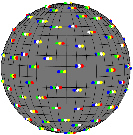
Recently, a slab-selective RF-encoded acquisition method called gSlider1 has been proposed to significantly improve spatial resolution along the slice dimension in diffusion MRI. In this approach, the thin slices within a thick slab are spatially-encoded using different spatially-selective RF pulses across multiple acquisitions, and an image with high-resolution along the slice dimension is estimated from the differently-encoded thick-slab images by solving a simple least-squares inverse problem. This approach enables highly-efficient high-resolution diffusion imaging, although further accelerations would still be desirable. To reduce gSlider sampling requirements and improve acquisition speed even further, some authors2,3 have proposed to subsample the gSlider (diffusion, RF)-encoding space in an interlaced way, where only a subset of RF encodings is observed at each location in q-space, while the subset of measured RF encodings varies from location to location. This type of scheme is illustrated in Figure 1. Subsequently, q-space regularization strategies can be used to compensate for the missing data. However, different authors have used different regularization strategies (Ref. 2 used Laplace-Beltrami quadratic smoothness regularization4 while Ref. 3 used spherical ridgelet sparsity regularization5), and the relative advantages and disadvantages of these two strategies are not obvious. In this work, we systematically compare these two regularization strategies and evaluate their potential synergies.Methods
OptimizationFormulation To evaluate the different regularization strategies, we consider a gSlider formulation that combines both penalties together:
$$ \hat{\mathbf{x}} = \arg\min_{\mathbf{x}} \frac{1}{2} \| \mathbf{b} - \mathbf{A}\mathbf{x} \|_2^2 + \beta R(\mathbf{x}) + \lambda L(\mathbf{x}).$$
Here, $$$\mathbf{x}$$$ is the vector of high-resolution image values (unknown and to be estimated) for all of the different diffusion encodings, $$$\mathbf{b}$$$ is the vector of measured thick-slab data for all of the different RF encodings and diffusion encodings, $$$\mathbf{A}$$$ is the operator that models gSlider data acquisition with interlaced subsampling, $$$R(\cdot)$$$ is an $\ell_1$-norm regularization penalty that promotes sparsity of the spherical ridgelet coefficients of the estimated data3,5, and $$$L(\cdot)$$$ is an $$$\ell_2$$$-norm Tikhonov Laplace-Beltrami regularization penalty that promotes smoothness of the estimated data2,4. The regularization parameters $$$\beta$$$ and $$$\lambda$$$ respectively control the strength of the spherical ridgelet and Laplace-Beltrami regularization terms.
This optimization problem was solved using the FISTA algorithm7.
Using this formulation, simulated gSlider data was reconstructed with systematic variation of the $$$(\lambda, \beta)$$$ parameters to elucidate the characteristics of the different regularization methods. The case with $\lambda=0$ yields Laplace-Beltrami regularization by itself, and the case with $$$\beta=0$$$ yields spherical ridgelet regularization by itself. Both regularization penalties are active when both $$$\lambda$$$ and $$$\beta$$$ are nonzero.
Simulations
Four-average gSlider data with 860 $$$\mu m$$$ isotropic resolution were acquired and combined to get a high quality reference dataset. For each average, the scan time is about 20 min. Interlaced subsampling was simulated as illustrated in Figure 1 where 3 or 4 RF encodings were acquired at each position in q-space out of 5 nominal RF encodings (the average was 3.5 RF encodings per q-space location, which corresponds to an acceleration factor of 1.4).
Evaluation Metrics
We computed normalized root mean square error (NRMSE) metrics for the recovered diffusion weighted images (DWIs) and for the quantitative fractional anisotropy (FA) estimate obtained from diffusion tensor fitting. We also calculated NRMSE metrics for two different orientation distribution function estimation methods: the Funk-Radon Transform (FRT)4 and the Funk-Radon and Cosine Transform (FRACT)6. These regularization strategies may behave differently for tissues with different anisotropy characteristics (e.g., gray matter and white matter), so we separated the image into components with high anisotropy (FA > 0.3) and low anisotropy (FA < 0.3) and report error metrics separately for each.
Results
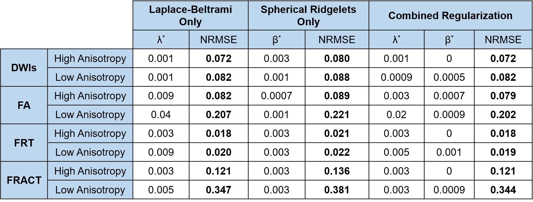
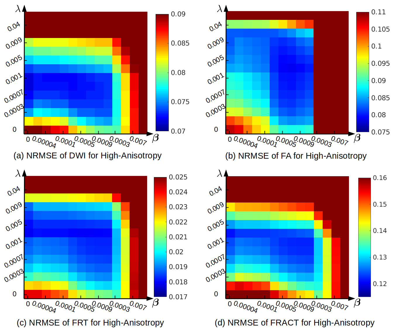
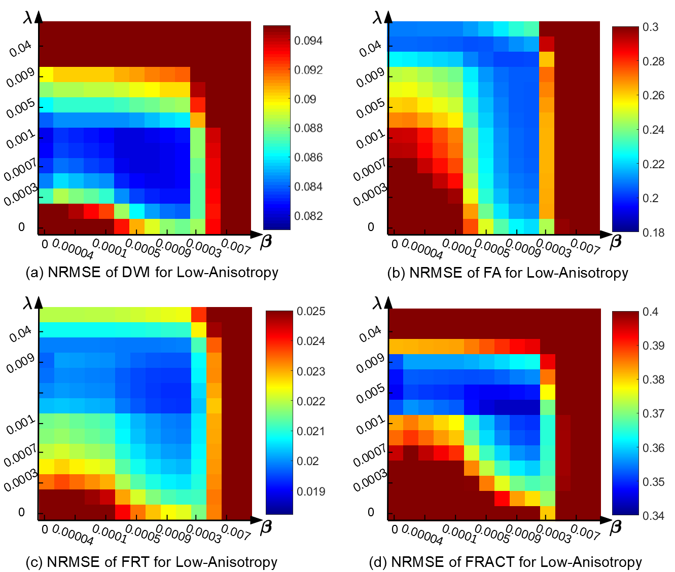
Quantitative results are shown in Figures 2-4. We observe that Laplace-Beltrami regularization by itself was consistently better than spherical ridgelet regularization by itself for all error metrics, although differences were often small. Combining different regularization strategies together often yielded further performance improvements, although these were again small.Interestingly, different error metrics were associated with different optimal regularization parameters. Further, the optimal regularization parameters were also substantially different for the low-anisotropy and high-anisotropy voxels. This suggests that when such regularization is used in practical diffusion MRI applications, regularization parameters may need to be chosen carefully based on the objectives of the specific study.
Notably, Laplace-Beltrami regularization by itself leads to a simple linear least-squares problem that has an analytical closed-form solution that is easy to implement, while spherical ridgelet regularization or a combination of Laplace-Beltrami with spherical ridgelet regularization is nonlinear and requires iterative optimization. As a result, Laplace-Beltrami regularization by itself may be preferred if computational complexity is a concern.
Conclusion
Laplace-Beltrami smoothness regularization and spherical ridgelet sparsity regularization are both effective for reconstructing subsampled gSlider data and are complementary to one another. However, the differences we observed were relatively small, and Laplace-Beltrami regularization by itself may also be an attractive option because of its relative simplicity. Although we considered q-space regularization by itself in this work, it is likely that additional benefits would be obtained from combining q-space regularization with spatial regularization2,3,8. In addition, although this work specifically considered gSlider reconstruction, the results are likely applicable to other diffusion MRI acquisitions that also rely on interlaced subsampling9-11.Acknowledgements
This work was supported in part by research grants NSF CCF-1350563, NIH R01-MH116173, NIH R01-NS074980, and NIH R01-NS089212, as well as a USC Viterbi/Graduate School Fellowship.References
[1] Setsompop K, Fan Q, Stockmann J, Bilgic B, Huang S, Cauley SF, Nummenmaa A, Wang F, Rathi Y, Witzel T, Wald LL. “High-resolution in vivo diffusion imaging of the human brain with generalized slice dithered enhanced resolution: Simultaneous multislice (gSlider-SMS).” Magnetic Resonance in Medicine 79:141-151, 2018.
[2] Haldar JP, Setsompop K. “Fast high-resolution diffusion MRI using gSlider-SMS, interlaced subsampling, and SNR-enhancing joint reconstruction.” Proc. ISMRM 2017, p. 175.
[3] Ramos-Llorden G, Ning L, Liao C, Mukhometzianov R, Michailovich O, Setsompop O, Rathi Y. “High-fidelity, accelerated whole-brain submillimeter in-vivo diffusion MRI using gSlider-spherical ridgelets (gSlider-SR).” Preprint arXiv:1909.07925, 2019.
[4] Descoteaux M, Angelino E, Fitzgibbons S, Deriche R. “Regularized, fast, and robust analytical q-ball imaging.” Magnetic Resonance in Medicine 58:497-510, 2007.
[5] Michailovich O, Rathi Y. “On approximation of orientation distributions by means of spherical ridgelets.” IEEE Transactions on Image Processing 19:461-477, 2010.
[6] Haldar JP and Leahy RM. “Linear transforms for Fourier data on the sphere: Application to high angular resolution diffusion MRI of the brain.” NeuroImage 71:233-247, 2013.
[7] Beck A and Teboulle M. “A fast iterative shrinkage thresholding algorithm for linear inverse problems,” SIAM Journal on Imaging Science 2:183–202, 2009.
[8] Haldar JP, Fan Q, and Setsompop K. “Fast sub-millimeter diffusion MRI using gSlider-SMS and SNR-enhancing joint reconstruction,” arXiv:1908.05698, 2019.
[9] Bhushan C, Joshi AA, Leahy RM, and Haldar JP. “Improved B0-distortion correction in diffusion MRI using interlaced q-space sampling and constrained reconstruction,” Magnetic Resonance in Medicine 72:1218–1232, 2014.
[10] Steenkiste GV, Jeurissen B, Veraart J, den Dekker AJ, Parizel PM, Poot DH, and Sijbers J. “Super-resolution reconstructionof diffusion parameters from diffusion-weighted images with different slice orientations,” Magnetic Resonance in Medicine 75:181–195, 2016.
[11] Ning L, Setsompop K, Michailovich O, Makris N, Shenton ME, Westin CF, and Rathi Y. “A joint compressed sensing and super-resolution approach for very high-resolution diffusion imaging,” NeuroImage 125:386 – 400, 2016.
Figures