4366
Regularized Image Domain Split Slice-GRAPPA for Simultaneous Multi-Slice Diffusion MR Imaging1Electrical and Computer Engineering, University of Utah, SALT LAKE CITY, UT, United States, 2Radiology and Imaging Science, University of Utah, SALT LAKE CITY, UT, United States, 3Biomedical Engineering, University of Utah, SALT LAKE CITY, UT, United States
Synopsis
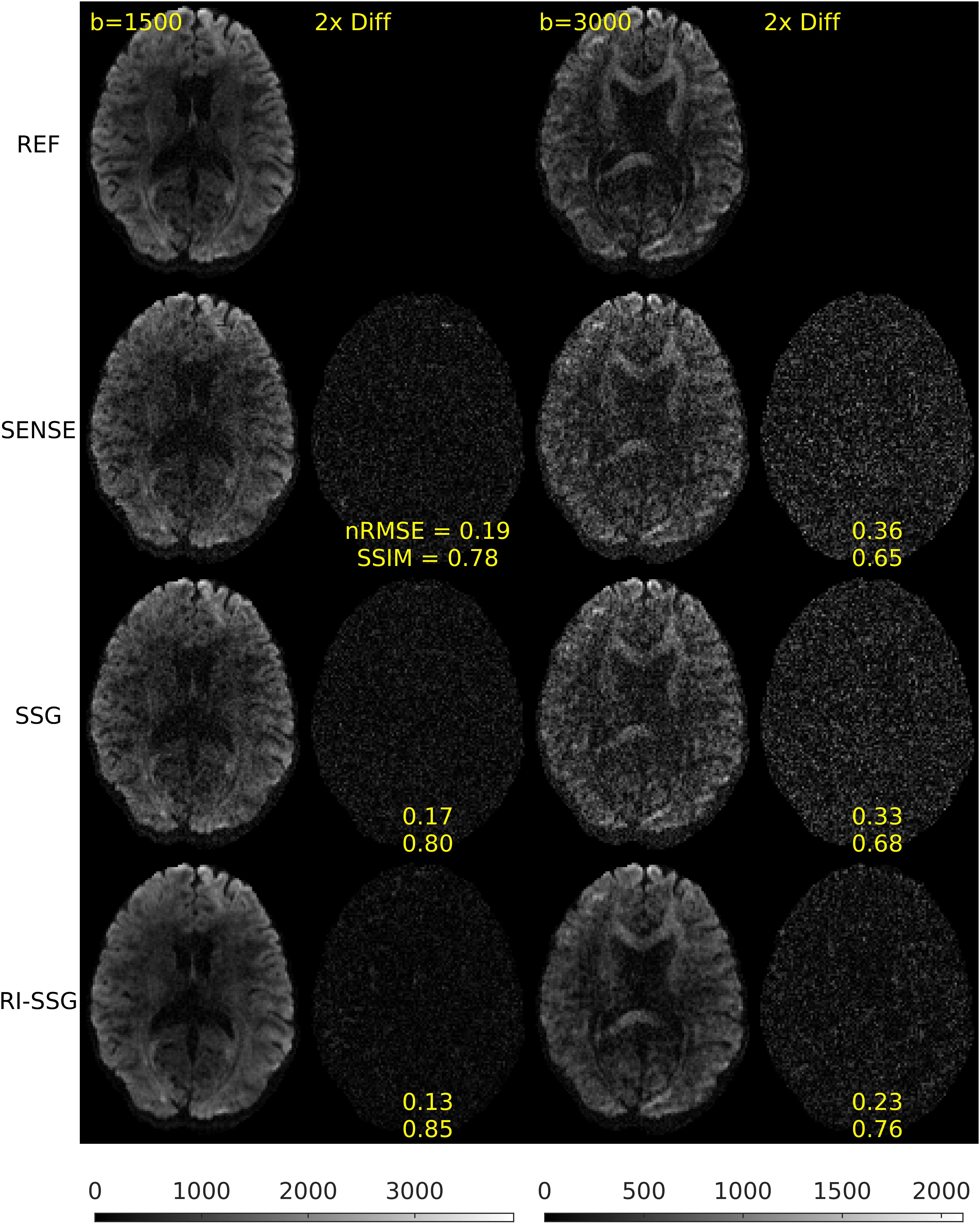
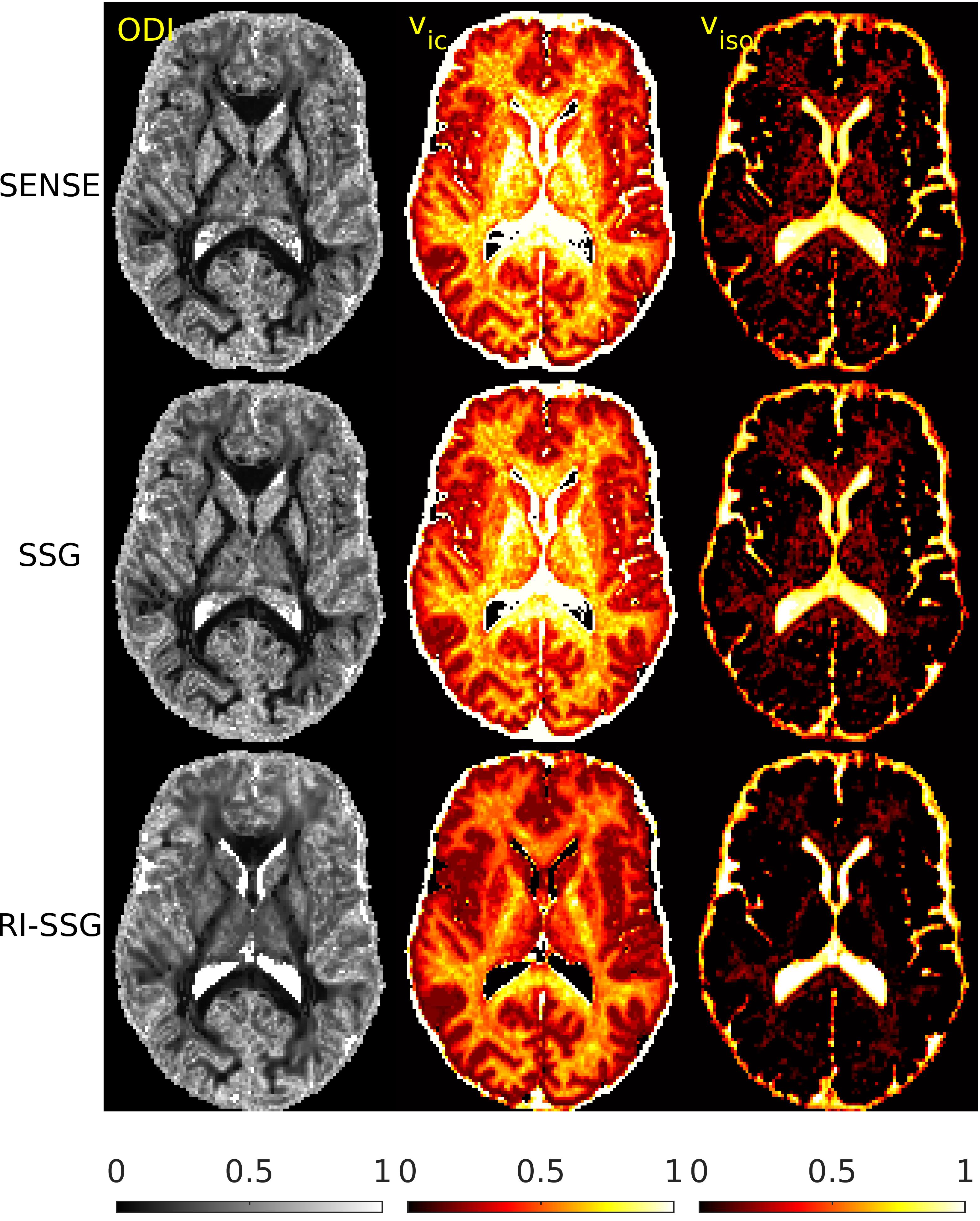
Simultaneous multi-slice (SMS) acquisition combined with blipped controlled aliasing in parallel imaging is commonly used to accelerate diffusion imaging with single-shot EPI sequences. In this work, we propose a new method, termed regularized image domain split slice-GRAPPA (RI-SSG), which allows an efficient image domain implementation of SSG coupled with total variation regularization to improve the quality of SMS reconstruction. We process two single-shot EPI datasets acquired using diffusion protocol of Human Connectome Project in Aging to evaluate performance of SMS reconstructions. The RI-SSG yields less noisy results than SENSE and SSG in estimating diffusion-weighted images and parametric maps of diffusion.
Introduction
Simultaneous multi-slice (SMS) acquisition combined with blipped controlled aliasing in parallel imaging (CAIPI)[1] is commonly used to accelerate diffusion imaging with single-shot EPI sequences. Sensitivity encoding (SENSE)[2] in image domain and slice-GRAPPA (SG)[1] in k-space are the basis for the most SMS reconstruction methods. In this work, we propose a new method, termed regularized image domain split slice-GRAPPA[3] (RI-SSG), which allows an efficient image domain implementation of SSG coupled with total variation (TV) regularization to improve the quality of SMS reconstruction for the estimation of diffusion-weighted images (DWIs) and parametric maps of diffusion.Theory
Suppose that a set of multi-coil and multi-slice DWIs with $$$z = 1,\cdots,N_s$$$ simultaneous slices, $$$n=1,\cdots,N_d$$$ diffusion directions, and $$$i=1,\cdots,N_c$$$ coils are acquired. These DWIs which are the IFFT of k-space data are written as$$m_{i,z,n}(x,y) =c_{i,z}(x,y)s_{z,n}(x,y), \quad (1)$$
where $$$(x,y)$$$ is pixel position, $$$s_{z,n}$$$ is the underlying magnetization image, and $$$c_{i,z}$$$ is the coil sensitivity. Assume that single slices are phase modulated using blipped-CAIPI[1], with superscript $$$(\phi_z)$$$ denoting phase modulation of slice $$$z$$$. Then, for the SMS image we have
$$r_{i,n}(x,y) =\sum_{z=1}^{N_s}m_{i,z,n}^{(\phi_z)}(x,y).\quad (2)$$
The SSG reconstruction using image domain kernels are described with following equations:
$$\widehat{m}_{i,z,n}^{(\phi_z)}(x,y) =\sum_{j=1}^{N_c} k_{i,z,j}(x,y)r_{j,n}(x,y). \quad (3)$$
By substituting (2) into (3) and separating slice of interest $$$z$$$ from other slices, we obtain
$$\widehat{m}_{i,z,n}^{(\phi_z)}(x,y) =\sum_{j=1}^{N_c}k_{i,z,j}(x,y)m_{j,z,n}^{(\phi_z)}(x,y)\\+\sum_{j=1}^{N_c}\sum_{z'=1,z'\neq z}^{N_s}k_{i,z,j}(x,y)m_{j,z',n}^{(\phi_{z'})}(x,y).\quad (4)$$
In the proposed RI-SSG, by assuming that kernels are slowly varying and hence by approximating them as piece-wise constant functions on small local neighborhoods (e.g., rectangular patches), we can solve (4) for kernel coefficients $$$k_{i,z,j}$$$. To control intra-slice artifacts and inter-slice leakages simultaneously, we let the first summation in (4) equal to $$$\widehat{m}_{i,z,n}^{(\phi_z)}(x,y)$$$ and the second summation be zero. For kernel training, we use (4) with b=0 images ($$$n=0$$$).Therefore, RI-SSG kernel training on a local patch $$$\Omega$$$ is written as
$$\begin{pmatrix} \vdots \\ \mathbf{0}\\ \mathbf{m}_{i,z,0}\\ \mathbf{0}\\ \vdots \end{pmatrix} = \begin{pmatrix} \mathbf{m}_{1,1,0} & \dots & \mathbf{m}_{N_c,1,0}\\ \vdots & \ddots &\vdots \\ \mathbf{m}_{1,z,0} & \dots & \mathbf{m}_{N_c,z,0} \\ \vdots & \ddots & \vdots \\ \mathbf{m}_{1,N_s,0} & \dots & \mathbf{m}_{N_c,N_s,0} \end{pmatrix} \begin{pmatrix} {k}_{i,z,1} \\ {k}_{i,z,2} \\ \vdots \\ {k}_{i,z,N_c} \end{pmatrix}\quad (5)$$
where $$$\mathbf{m}_{i,z,0}$$$ is the vectorized form of $$$\{m_{i,z,0}^{(\phi_z)}(x,y)|(x,y)\in\Omega\}$$$. Equation (5) is well conditioned when $$$|\Omega|\times N_s \gg N_c$$$. After kernel training, SMS reconstruction using RI-SSG is formulated as
$$\{\mathbf{s}_{z,n}^{\star}|_{z=1}^{N_s}|_{n=1}^{N_d}\} = \arg\min_{\{\mathbf{s}_{z,n}|_{z=1}^{N_s}|_{n=1}^{N_d}\}} \sum_{n=1}^{N_d}\sum_{z'=1}^{N_s} \left\| \overbrace{\sum_{i}\mathbf{c}_{i,z'}^{*}}^{\text{(C)}}\overbrace{\sum_{j}k_{i,z',j}}^{\text{(B)}}\overbrace{\mathbf{r}_{j,n}}^{\text{(A)}}-\overbrace{\sum_{i}\mathbf{c}_{i,z'}^{*}}^{\text{(C)}}\overbrace{\sum_{j}k_{i,z',j}}^{\text{(B)}}\overbrace{\sum_{z}\mathbf{c}_{j,z}\mathbf{s}_{z,n}}^{(\text{A}')}\right\|_2^2 \\+ \lambda\sum_{n=1}^{N_d}\sum_{z=1}^{N_s} \left( \left\|\nabla_x(\mathbf{s}_{z,n})\right\|_1 + \left\|\nabla_y(\mathbf{s}_{z,n})\right\|_1\right),\quad (6)$$
where $$$\mathbf{s}_{z,n}$$$, $$$\mathbf{c}_{i,z}$$$, and $$$\mathbf{r}_{j,n}$$$ are the vectorized form of $$$\{s_{z,n}^{(\phi_z)}(x,y)|(x,y)\in\Omega\}$$$, $$$\{c_{i,z}^{(\phi_z)}(x,y)|(x,y)\in\Omega\}$$$, and $$$\{r_{j,n}(x,y)|(x,y)\in\Omega\}$$$, respectively. We solve (6) independently for each $$$ \Omega$$$ to jointly estimate all simultaneous single slices. Directions can be reconstructed one at a time, or, with (6) regularization across directions could be included. The first term in (6) enforces data consistency, where (A) denotes acquired SMS images, (A') is the forward model using (1) and (2), (B) is de-aliasing of SMS images using RI-SSG kernels, and (C) is sensitivity-weighted coil combining. The second term imposes TV regularization on estimated single slices. The weighting parameter $$$\lambda$$$ adjusts trade-off between the two constraints.
Methods
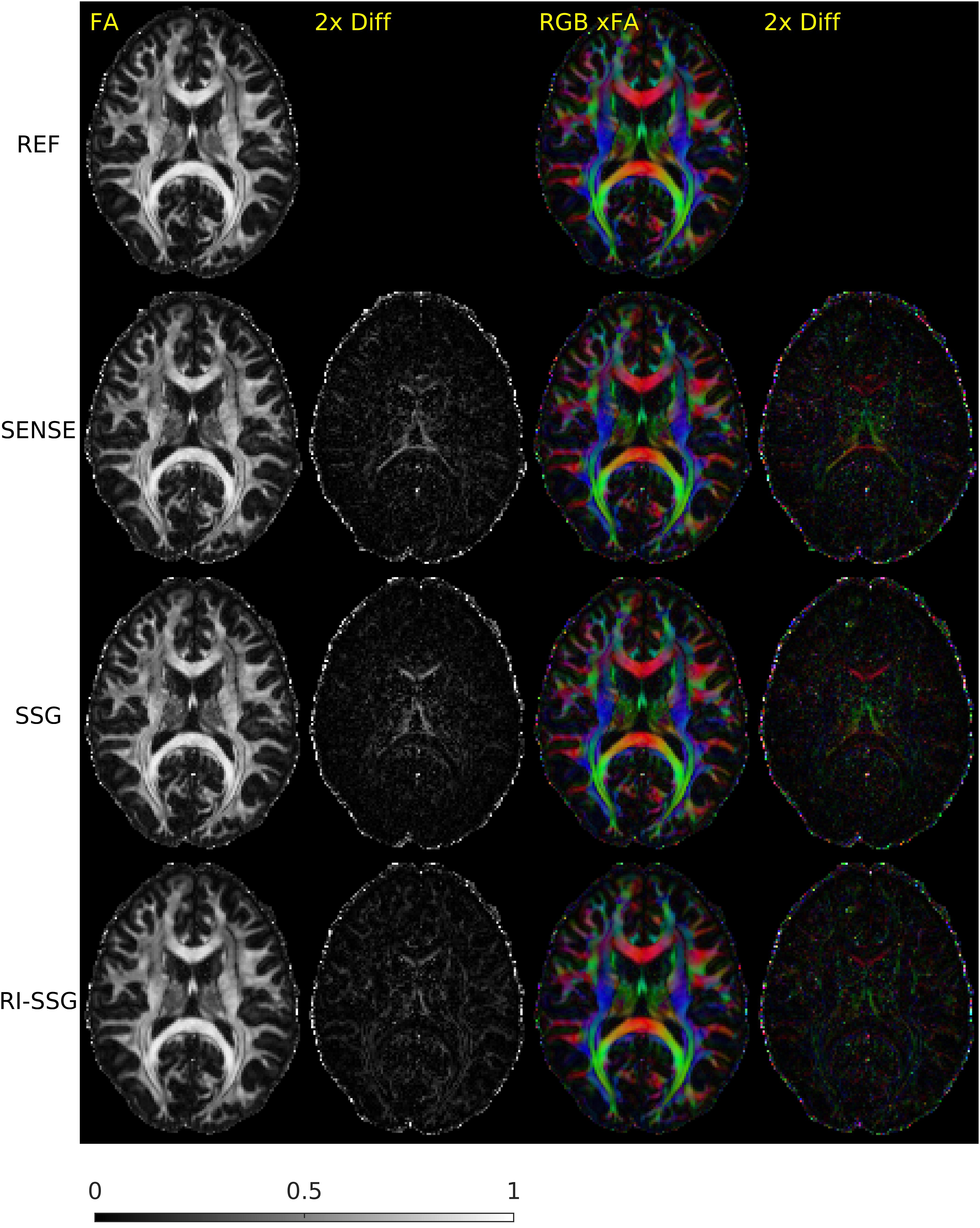
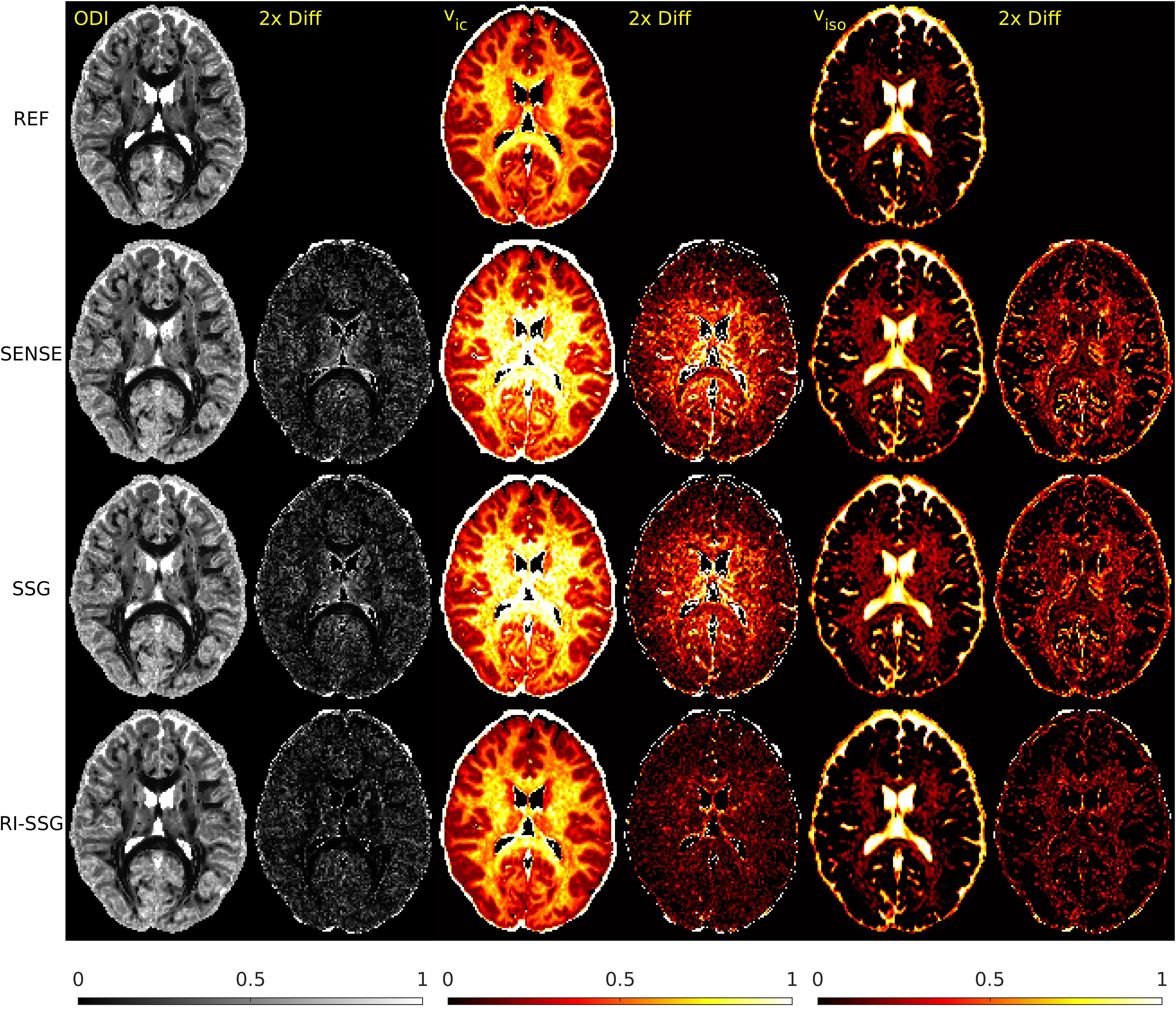
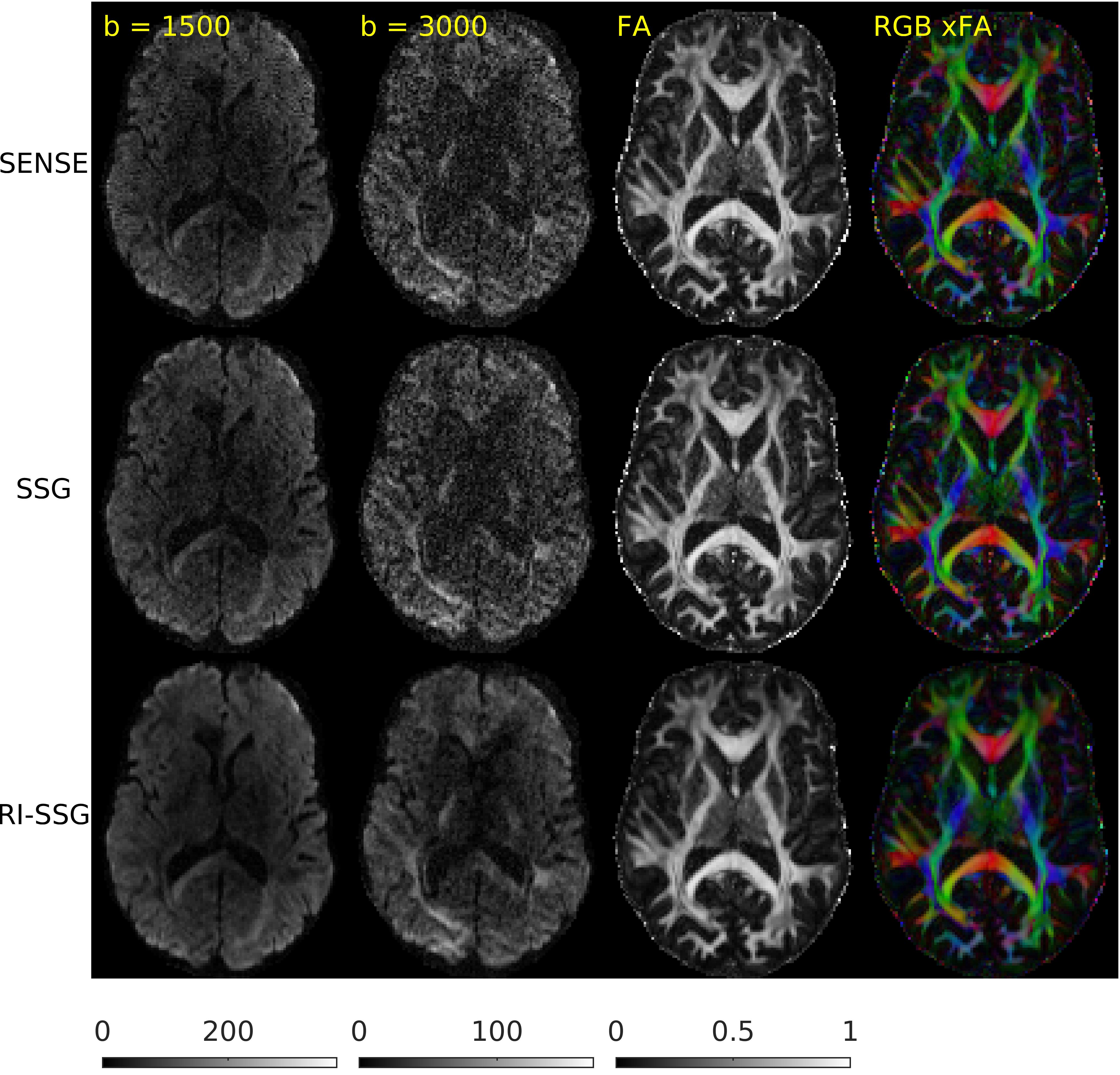
Two single-shot EPI diffusion datasets were acquired using a Siemens 3T Prisma scanner from a normal volunteer and a stroke patient with informed consent and IRB approval. The first dataset was acquired without slice acceleration and SMS acquisition with $$$N_s$$$=4 was simulated subsequently. A 32-channel head coil was used to acquire two sessions of the diffusion protocol of Human Connectome Project in Aging (HCP-A)[4] with AP and PA phase-encoding. In each session, we acquired seven b=0, 46 DWIs of b=1500 s/mm$$$^2$$$, and 46 DWIs of b=3000 s/mm$$$^2$$$, with TE = 83.8 ms, TR = 13194 ms, number of slices = 92, voxel size = 1.5$$$\times$$$1.5 $$$\times$$$1.5 mm$$$^3$$$, matrix size = 140$$$\times$$$105, and partial Fourier 6/8. The second dataset was acquired with $$$N_s$$$=4, a 64-channel head coil, TE = 89.2 ms, TR = 3230 ms, number of slices = 23$$$\times$$$4. Other acquisition settings were the same as the first dataset. Each session took ~22 minutes for the first dataset, and ~5 minutes for the second dataset. Whitening of noise and EPI phase corrections were performed prior to SMS reconstructions. A single band non-diffusion scan was used for kernel training and sensitivity estimations. SMS reconstruction was performed using SENSE, SSG, and RI-SSG. For SSG k-space kernel sizes were 7$$$\times$$$7. For RI-SSG we set $$$\Omega$$$ to be 12$$$\times$$$12 patches with stride of 4 and reconstruction results in overlapping areas were averaged. Setting $$$\lambda$$$=10$$$^{-6}$$$, Projection onto Convex Sets (POCS)[5] was used to solve (6) with maximum number of iterations 10, and relaxation parameters of 0.075 and 0.1 for data fidelity and TV regularization, respectively. SMS reconstruction in image domain was evaluated using magnitude DWIs. Prior to model fitting, DWIs were processed using a pipeline consisting of ringing artifact removal, EPI susceptibility distortions correction (topup)[6], eddy current and subject motion corrections[6]. Model fitting was done using a standard approach[7] for DTI, and using accelerated microstructure imaging via convex optimization (AMICO)[8] for neurite orientation dispersion and density imaging (NODDI).Results
The SMS reconstruction results for the two datasets are shown in Figures 1-3 and Figures 4-5, respectively.Conclusions
In this work, we proposed a novel regularized image domain SSG method (RI-SSG) for SMS reconstruction that demonstrated less noisy DWIs and more accurate diffusion parametric maps than SENSE and SSG.Acknowledgements
We thank Dr. Douglas Dean and Dr. Andrew Alexander for providing the diffusion processing pipeline and Darshan Shimpi for his assistance with the processing pipeline.References
[1] Setsompop K., et al., Blipped-controlled aliasing in parallel imaging for simultaneous multi-slice echo planar imaging with reduced g-factor penalty. Magnetic Resonance in Medicine, 67(5):1210–1224, 2012.
[2] Larkman David J., et al., Use of multi-coil arrays for separation of signal from multiple slices simultaneously excited. Journal of Magnetic Resonance Imaging, 13(2):313–317, 2001.
[3] Cauley S. F., et al., Inter-slice leakage artifact reduction technique for simultaneous multi-slice acquisitions. Magnetic Resonance in Medicine, 72(1):93–102, 2014.
[4] Harms Michael P., et al., Extending the human connectome project across ages:Imaging protocols for the lifespan development and aging projects. NeuroImage, 183:972 – 984, 2018.
[5] Samsonov Alexei A., et al., Pocsense:Pocs-based reconstruction for sensitivity encoded magnetic resonance imaging. Magnetic Resonance in Medicine, 52(6):1397–1406, 2004.
[6] Jenkinson Mark, et al., Fsl. NeuroImage, 62(2):782 – 790, 2012. 20 YEARS OF fMRI.
[7] Garyfallidis Eleftherios, et al., Dipy, a library for the analysis of diffusion MRI data. Frontiers in Neuroinformatics, 8:8, 2014.
[8] Daducci Alessandro, et al., Accelerated microstructure imaging via convex optimization (AMICO) from diffusion MRI data. NeuroImage, 105:32 – 44, 2015.
Figures