INTRODUCTION

Diffusion-weighted magnetic resonance imaging (DWI) is a widely used neuroimaging technique to study brain microstructure and connectivity. Advanced diffusion signal models such as multi-compartmental models can provide pathologically relevant biomarkers for studying disease progression in the brain. However, to probe tissue microstructure using such models and to resolve the ambiguities in the parameters related to tissue microstructure, the acquisition of diffusion MRI (dMRI) data at high spatial resolution and on a large number of q-space points (high angular resolution) are needed¹.

Here, we propose to utilize an efficient sampling scheme and a novel reconstruction method to address the high acquisition demands of such data and the complex reconstruction involved. Specifically, we propose a model-based deep learning architecture for the reconstruction of highly accelerated dMRI that enables high-resolution imaging.

METHODS

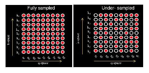
To achieve high spatial and angular resolution, we utilize a multi-shot k-space sampling scheme for sampling a large number of diffusion directions. Since such a fully sampled acquisition takes prohibitively long scan time, we employ a joint k-q under-sampling scheme² to reduce the scan time. Figure 1 demonstrate the proposed scheme which has been shown to afford high acceleration factors compared to traditional under-sampling schemes².

Since the data is highly under-sampled in both the k-q dimension, we develop a joint reconstruction to recover all the DWIs in a single step. Note that the above reconstruction also needs to account for the phase variations associated with the multi-shot acquisition. A standard parallel imaging-only reconstruction, with phase compensation, is not adequate to recover such highly under-sampled data. Previously, fingerprinting-like methods that relied on a dictionary of diffusion parameters have been used in combination with l₁-based priors^2,3,4 to develop under-sampled recovery schemes. However, the extension of this approach for the case of multi-compartmental models is highly computationally expensive due to the high number of model parameters involved. Hence, instead of relying on dictionary matching, we develop a novel prior based on deep learning to enable the joint recovery of such data.

Specifically, we introduce a self-learning dMRI framework based on de-noising autoencoders (DAE) that learn the data manifold of the diffusion signal in q-space. To perform the learning, we make use of the 3-compartment model for diffusion signals, given by:
\begin{equation}
S(b,~\mathbf{g})~=~S_0\int_{\hat{ \bf{n}}}~{\cal{P}}(\hat{ \bf{n}})~\circledast~K(b,\hat{\bf{g}}~\cdot~\mathbf n)~d\hat{\bf{n}}~~~~~~~~(1)
\label{model}
\end{equation}
Here, $$$\mathcal{P}$$$ is the fiber orientation distribution function and $$$\circledast$$$ denotes a spherical convolution operation with a kernel $$$K$$$, given by
\begin{equation}
\hspace{0em}
K(b,\zeta)~=~f_1e^{-bD_a\zeta^2}~+~f_2e^{-bD_e^{\perp}~-b\left(D_e^{||}~-~D_e^{\perp}\right)\zeta^2}+f_{\rm iso}~e^{-bD_{\rm iso}}.
\end{equation}
The microstructural parameters are the volume fractions denoted by $$$f_{i}$$$'s, and the compartmental diffusivities $$$D$$$'s. $$$b$$$ is the diffusion weighting, $$$S(b,~\mathbf~g)~$$$ and $$$S_0$$$ are the DWI and the reference image.

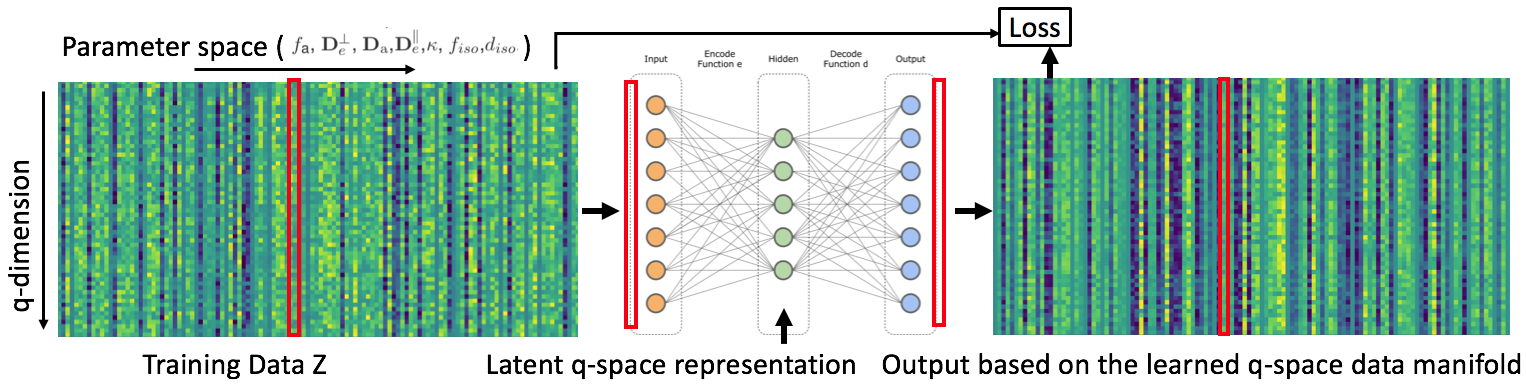
Using the above model, we generate diffusion signals, $$$S(b,~\mathbf{g})$$$, for a range of model parameters for a fixed set of q-space points. The diffusion signal generated along the q-space points are then used to train a DAE which learns the manifold. Figure 2 illustrates the above concept. Once the parameters Θ of the manifold are learned, we propose to use the residual error of DAE as a reconstruction prior. The final reconstruction that simultaneously performs phase correction and joint reconstruction of the msDWI from joint k-q under-sampled data is given by

\begin{equation}\label{joint}\mathbf{P^{*}}~=~\arg~\min_{\mathbf~P}~\|\mathcal~A~(\mathbf P)-\widehat{\mathbf{Y}}\|^{2}_{2}+~\lambda~\|\mathbf{P}~-~\mathcal~D_{\Theta}(\mathbf{P})\|^{2}~~~~~~~~(2)~\end{equation}
Here, $$$\mathbf{P}$$$ is the matrix of DWIs jointly recovered from all q-space points and $$$\mathcal{D}_{\Theta}(\mathbf~P)$$$ is the DAE trained using the data generated from a generalized diffusion model. $$$\mathbf{\hat{Y}}$$$ is the Casoratti matrix (of dimension $$$~N_1~\times~N_2~\times~\times N_s~\times~Q$$$), of the k-space data corresponding to the different q-space points and shots. $$$\mathcal{A}=\mathcal{S}_s\circ~\mathcal{F}~\circ~\mathcal~{C}~$$$ where, $$$\mathcal{F}, \mathcal{S}_s$$$, and $$$\mathcal{C}$$$ denote Fourier transform, k-space sampling mask for each shot $$$s$$$, and weighting by coil sensitivities, respectively. To accommodate phase compensation, the coil sensitivites are multiplied by the phase of the corresponding shot.

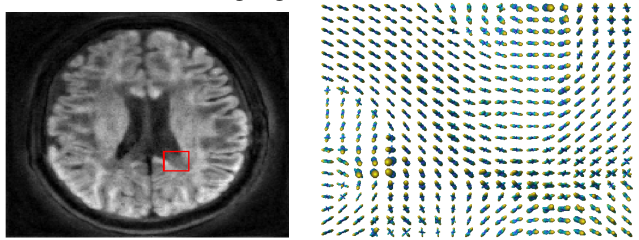
We solve the above optimization using the alternating direction method of multipliers. For testing, we used a synthesized brain MRI ground truth data shown in figure 3.

RESULTS

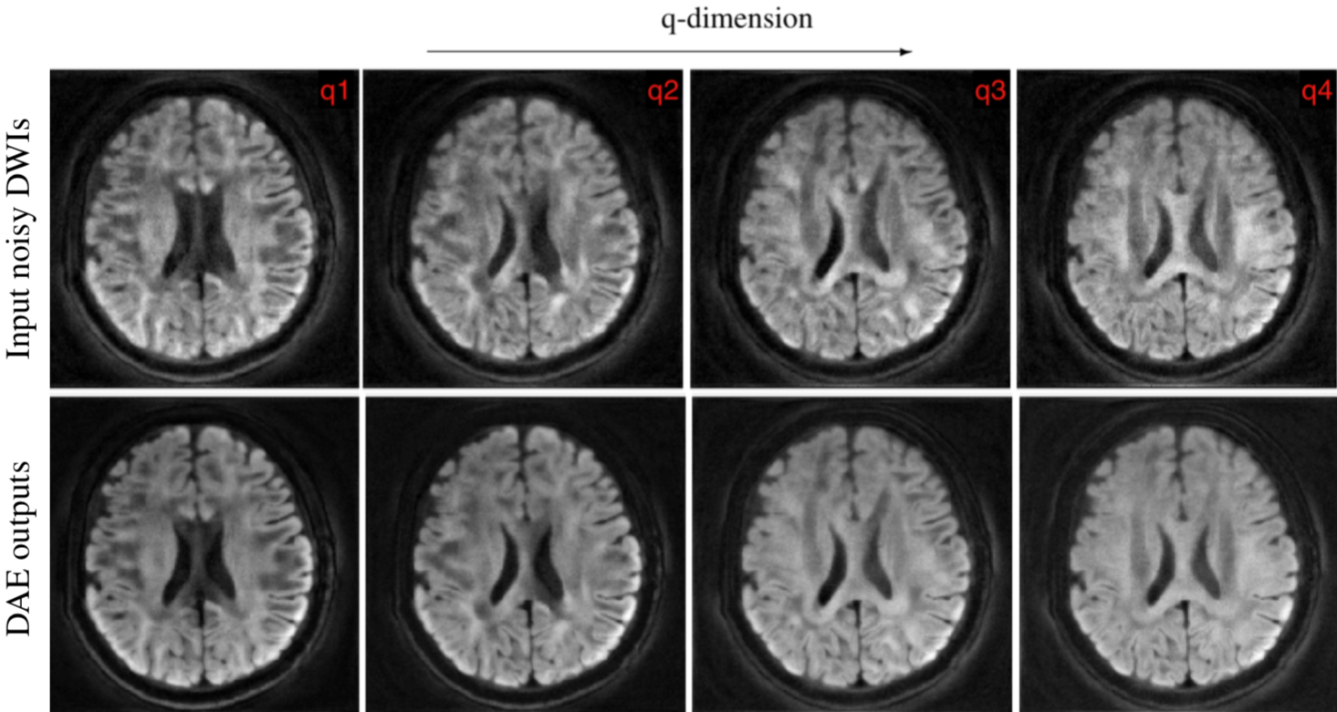
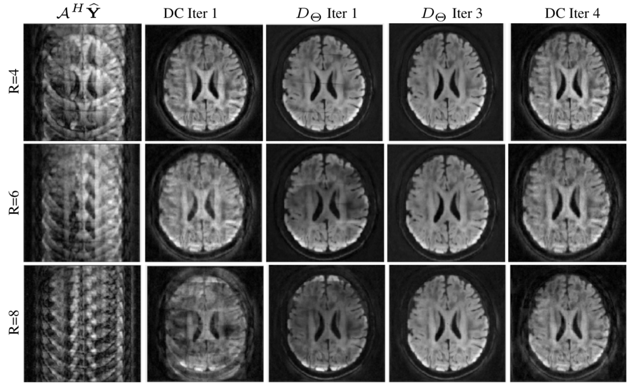
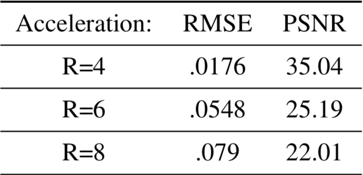
In Figure 4, we provide the testing results of the DAE. The figure shows the learned output of the DAE, which reconstructed the DWIs in a voxel-wise manner for noisy input data. Once the performance of the DAE were tested, we employed it for the joint recovery of highly under-sampled k-q data. The reconstruction results for various acceleration factors are shown in Figure 5. Here, 4-, 6- and 8-shot cases were tested. In all cases, only one random shot per q-space point was sampled corresponding to R=4,6 and 8. Table 1 reports the reconstruction error computed with respect to the ground truth data.

DISCUSSION AND CONCLUSIONS

Figure 4 shows the successful learning of the q-space signal manifold by the DAE. This is confirmed by the preservation of the diffusion contrast along the q-dimension in each voxel. Similarly, reconstruction results given in figure 5 and table 1 confirm the successful recovery of the DWIs at various under-sampling factors using the proposed scheme.

From the above results, it is evident that the proposed DAE regularizer is an efficient recovery prior that pre-learns the projection to the q-space signal manifold and aid the recovery of missing q-space data. In conclusion, we show the feasibility of employing a pre-learned DAE prior for recovering under-sampled dMRI data in a model-based recovery setting.

Acknowledgements

This work is supported by NIH 1R01EB019961-01A1.