4321
Optimal experimental design for multi-tissue spherical deconvolution of diffusion MRI1imec-Vision Lab, Dept. Physics, University of Antwerp, Antwerp, Belgium
Synopsis
Multi-tissue constrained spherical deconvolution of multi-shell diffusion weighted MRI data estimates the white matter fiber orientation distribution function, together with the densities of gray matter and cerebrospinal fluid. In this work, we propose a 5-minute scanning protocol that allows a more precise estimation of WM and GM densities, while maintaining a high angular resolution.
Introduction
Multi-tissue constrained spherical deconvolution (MT-CSD) of multi-shell diffusion weighted (DW) MRI data estimates the white matter fiber orientation distribution function (ODF), together with the densities of gray matter (GM) and cerebrospinal fluid (CSF)1. Currently, MT-CSD studies employ DW schemes with densely sampled shells with equidistant b-values2, or schemes with b-values optimized for diffusion kurtosis imaging1,3. In this work, we use the Cramér-Rao Lower Bound4 (CRLB) , which is a lower bound on the variance of any unbiased estimator. By minimizing the CRLB with respect to the b-values of all DW samples, we obtain a sampling scheme that allows a more precise estimation of the tissue densities. We propose an optimized 100-direction sampling scheme with a 5-minute scan time that allows a more precise estimation of WM and GM densities, while maintaining a high angular resolution.Methods
The forward DW signal model of MT-CSD can be written as:$$\boldsymbol{y}=A\boldsymbol{x}$$
with the vector $$$\boldsymbol{y}=\{y_1\;y_2\;...\;y_M\}^T$$$ containing the $$$M$$$ diffusion-weighted measurements, $$$A$$$ the $$$M$$$ by $$$N$$$ forward convolution matrix and $$$\boldsymbol{x}$$$ containing the spherical harmonics coefficients of the CSF, GM and WM ODFs. Assuming Gaussian noise with variance $$$\sigma^2$$$, the Fisher information matrix $$$F$$$ takes the form:
$$F=\frac{1}{\sigma^2}A^TA$$
A lower bound for the variance of $$$\boldsymbol{x}$$$ is given by the diagonal elements of the inverse of F, also known as the CRLB. Note that A depends on both the DW scheme and the tissue responses. The tissue responses, which themselves depend on the DW scheme, are modeled using a symmetric fourth order tensor model, for which the parameters were obtained from a densely sampled multi-shell data set. In order to find the optimal sampling scheme, we look for the set of b-values that minimize the CRLB of the tissue density estimators, ignoring the orientation information in the WM compartment. To further simplify the problem, the DW directions were fixed during the optimization (distributed on the half sphere using electrostatic repulsion). After obtaining the optimal b-values for each shell, electrostatic repulsion was again applied to the DW directions corresponding to each b-value , ensuring an isotropic distribution of directions for each shell.
We compared two DW schemes with 100 q-space samples and a total acquisition time of 5 minutes (TR = 2800ms, TE = 92ms, voxel size = 2.5 mm isotropic):
- Reference: a multi-shell scheme with equidistant b-values (b=0, 1000, 2000, 3000 s/mm2 in 10, 30, 30 and 30 directions respectively)
- Optimized: a CRLB-optimized scheme
Results
The CRLB-optimized scheme was found to contain three shells (b=0, 361, 3000 s/mm2 in 4, 24 and 72 directions, respectively), with the inner shell having a much lower b-value than that of the reference scheme. In addition, a greater amount of DW samples are placed in the outer shell, which will boost the angular information content.Fig. 1a shows the variance maps for WM, GM and CSF, estimated from simulations. A decrease in the variances can be seen for WM and GM densities, together with a slight increase in CSF density variance. Fig. 1b shows the distribution of the variances in Fig. 1a.
Fig. 2a depicts the tissue density variances estimated from the real data. Fig. 2b shows the distribution of the variances in Fig. 2a.
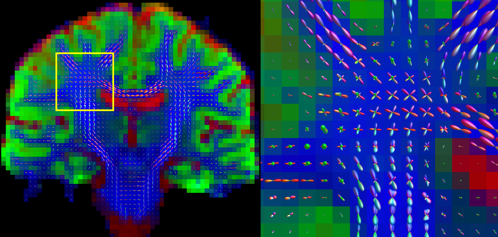
An example of the tissue densities and WM FODs estimated from data acquired with the optimized scheme can be appreciated in Fig. 3.
Discussion & Conclusion
In this work, we minimized the CRLB for WM, GM and CSF densities given a DW scheme with 100 q-space samples. Compared to a scheme with equidistant b-values, the optimized scheme allows for a more precise estimation of the WM and GM densities, coupled with a negligible reduction in CSF precision.Acknowledgements
No acknowledgement found.References
- Jeurissen B, Tournier J-D, Dhollander T, Connelly A, Sijbers J. Multi-tissue constrained spherical deconvolution for improved analysis of multi-shell diffusion MRI data. Neuroimage. 2014;103: 411–426.2.
- Kamath A, Aganj I, Xu J, Yacoub E, Ugurbil K, Sapiro G. Generalized constant solid angle ODF and optimal acquisition protocol for fiber orientation mapping.
- Poot DHJ, den Dekker AJ, Achten E, Verhoye M, Sijbers J. Optimal experimental design for diffusion kurtosis imaging. IEEE Trans Med Imaging. 2010;29: 819–829.4.
- van den Bos A. Parameter Estimation for Scientists and Engineers. Wiley-Interscience; 2007.
Figures

Figure 1: a) WM, GM and CSF density variance maps for 50 Rician noise realizations with reference and optimized DW schemes. Note that the CSF variance differences are an order of magnitude smaller than those of WM and GM. b) distribution of variances depicted in (a). The median variances of the maps shown in (a) are for the reference and optimized schemes, respectively: 9.20e-4 and 5.10e-4 (WM), 4.14e-4 and 1.92e-4 (GM), 1.67e-5 and 2.03e-5 (CSF).
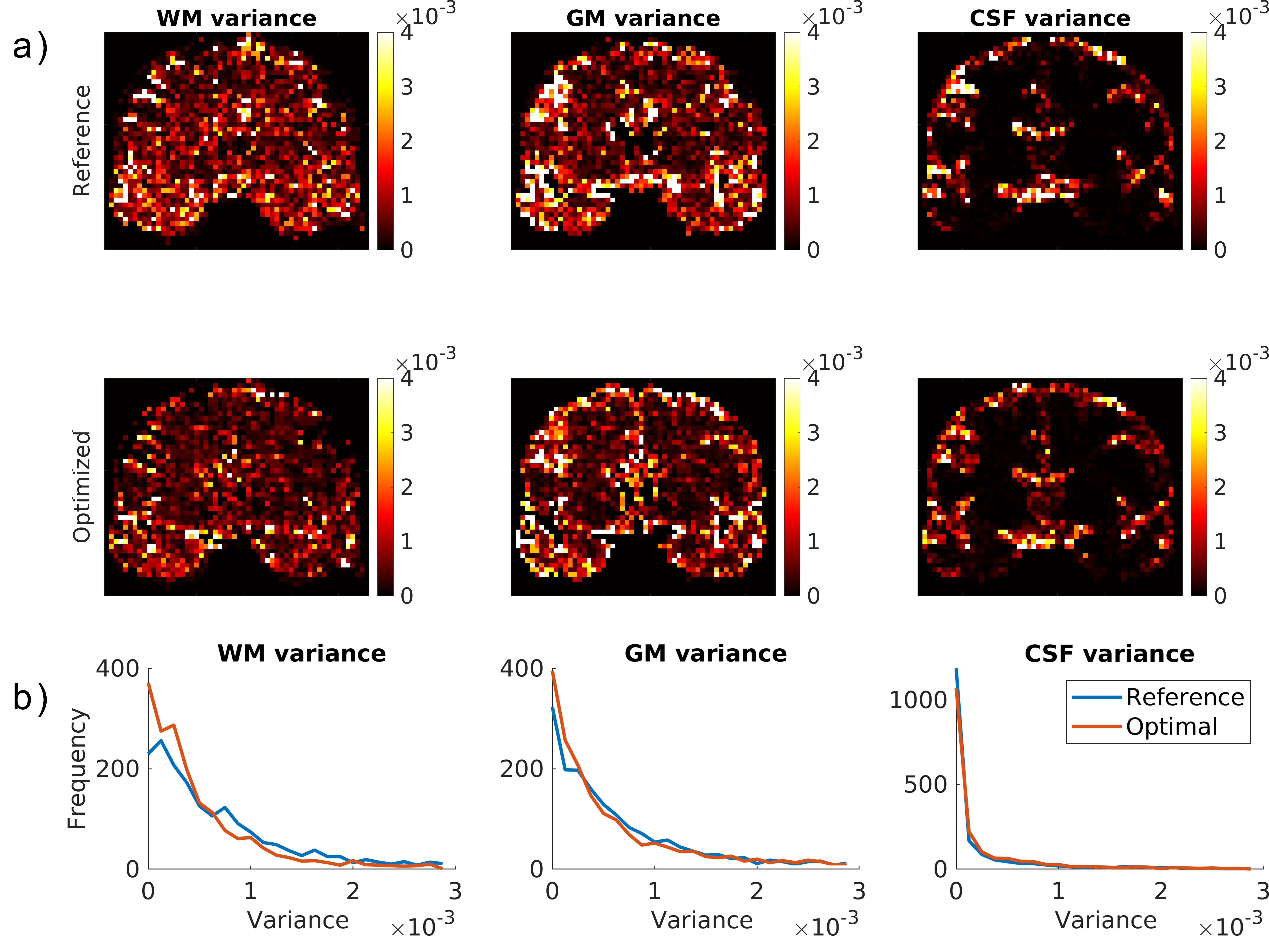
Figure 2: a) WM, GM and CSF density variance maps calculated from the real data acquired with the reference and optimized DW schemes. b) distribution of variances depicted in (a). The median variances of these maps are for the reference and optimized schemes, respectively: 5.58e-4 and 3.74e-4 (WM), 5.54e-4 and 4.38e-4 (GM), 5.00e-5 and 7.94e-5 (CSF).