Purpose

Diffusion MRI (dMRI) typically requires long acquisition time for probing water diffusion in various directions and scales. In this abstract, we propose to accelerate the acquisition via slice-interleaved diffusion encoding (SIDE), where only a subsample of slices are acquired for each diffusion wavevector, and demonstrate that it is possible to reconstruct the full DW volumes from highly slice-undersampled volumes using a GCNN.

Methods

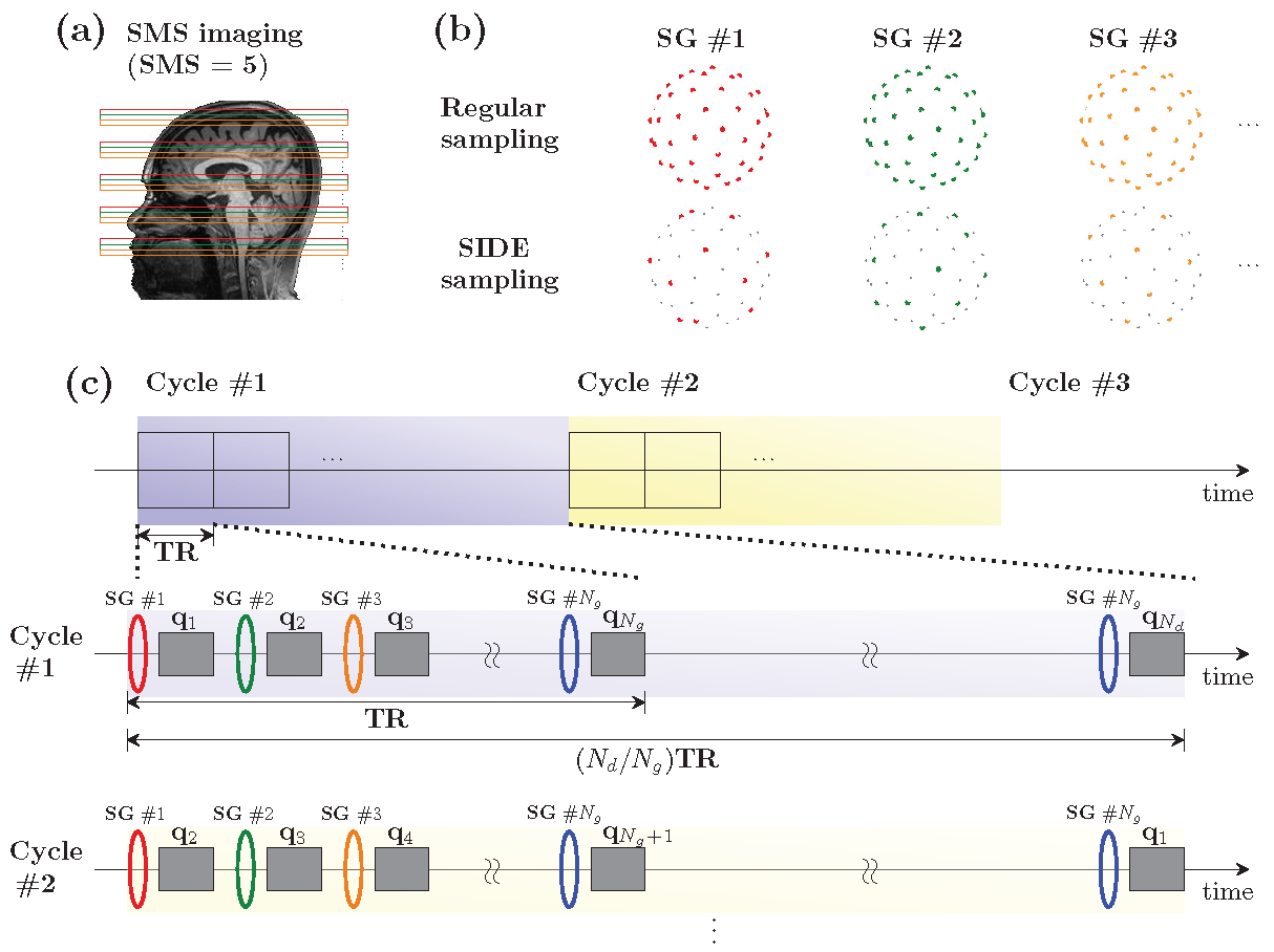
An example SIDE acquisition scheme is shown in Figure 1. Each simultaneous multi-slice (SMS) excitation is targeted at a slice group (SG) of 5 slices (Figure 1a). In conventional acquisition, all SGs in a volume share the same diffusion encoding (top row of Figure 1b). In contrast, SIDE allows the diffusion encodings of SGs in a volume to differ (bottom row of Figure 1b). Figure 1c illustrates that, in SIDE, the first SMS excitation is followed by the spin-echo EPI (SE-EPI) readout block with the first diffusion wavevector $$$\mathbf{q}_1$$$ in the gradient table. Likewise, the second SG is encoded by the second diffusion wavevector $$$\mathbf{q}_2$$$, and so forth.
Let $$$N_g$$$ denote the number of SGs in a volume and $$$N_d$$$ denote the number of wavevectors. Assuming $$$N_d$$$ is a multiple of $$$N_g$$$ for convenience, the first cycle of diffusion encoding will complete after $$$N_d/N_g$$$ TRs (middle row of Figure 1c). In the next cycle, the gradient table is offset by 1 so that the first SG in this cycle is encoded by the second gradient direction $$$\mathbf{q}_2$$$ (bottom row in Figure 1c). $$$N_g$$$ cycles cover all the slices of all diffusion wavevectors. A subset of the cycles can be selectively acquired based on a certain acceleration factor $$$R$$$.
Let $$$\{\tilde{X}_1, \cdots, \tilde{X}_{N_d}\}$$$ be the subsampled DW images, rearranged from the SIDE multi-wavevector volumes. Note that each $$$\tilde{X}_n$$$ is slice-undersampled by a factor of $$$R$$$. Our goal is to learn a non-linear mapping $$$f$$$ to reconstruct the full volumes from $$$\{\tilde{X}_1, \cdots, \tilde{X}_{N_d}\}$$$, i.e.,$$(X_1,\cdots,X_{N_d}) = f(\tilde{X}_1, \cdots, \tilde{X}_{N_d}),$$
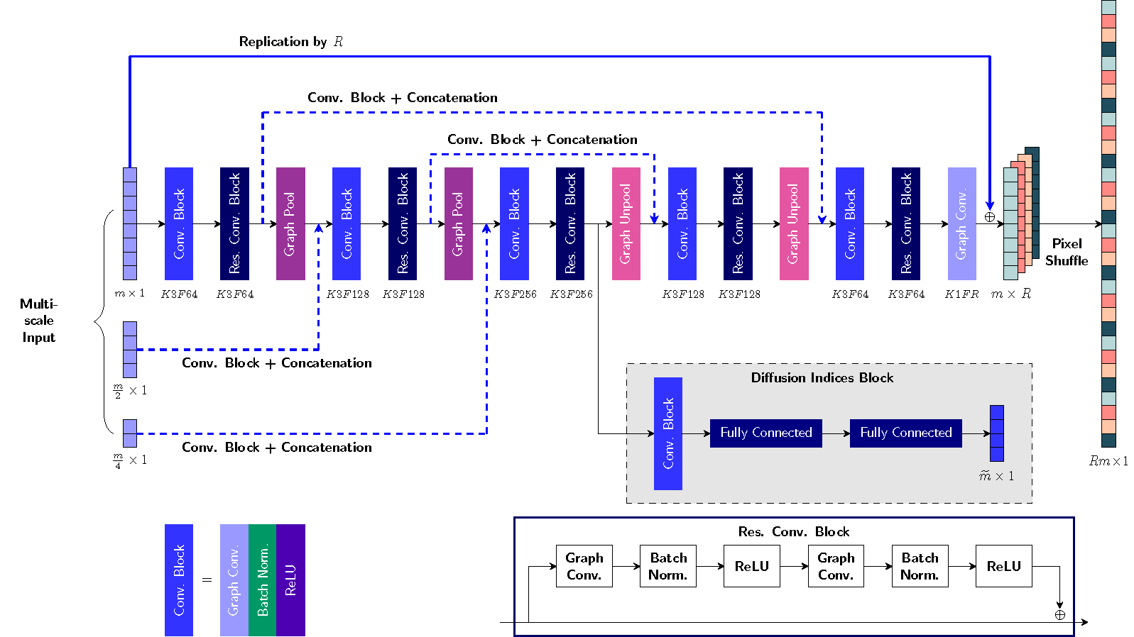
where $$$\{X_1,\cdots,X_{N_d}\}$$$ can be acquired after $$$N_g$$$ cycles. We employ a GCNN (Figure 2) to learn the mapping function, since dMRI data are not necessarily Cartesian-sampled in the wavevector space.

Materials

After obtaining informed consent, we acquired dMRI data from seven healthy subjects using a protocol approved by the institute and a 3T Siemens whole-body Prisma scanner (Siemens Healthcare, Erlangen, Germany). Diffusion imaging was performed with a monopolar diffusion-weighted SE-EPI sequence. The SMS RF excitation with controlled aliasing (blipped-CAIPI) was employed to reduce the penalty of geometry factor (g-factor). The SMS factor is 5. Imaging parameters were as follows: resolution= $$$1.5~ \text{mm}$$$ isotropic; FOV $$$= 192\times 192 \times 150 ~\text{mm}^3$$$; image dimensions $$$= 128\times 128\times 100$$$; partial Fourier = 6/8; no in-plane acceleration was used; bandwidth = 1776 Hz/Px; 160 wavevectors distributed over the 4 b-shells of $$$b = 500, 1000, 2000$$$ and $$$3000~ \text{s/mm}^2$$$, plus one $$$b=0$$$; TR/TE=3120/90 ms; 32-channel head array coil. The total acquisition time is 8 mins and 32 s for each phase-encoding direction. Note that $$$N_{d}$$$=160 and $$$N_{g}$$$=100/5=20.

Results

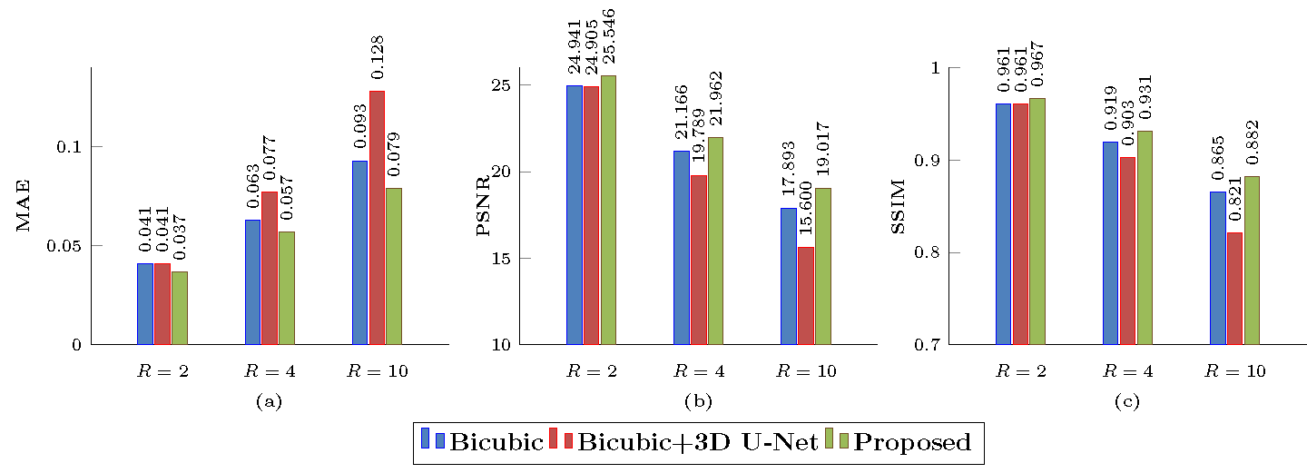
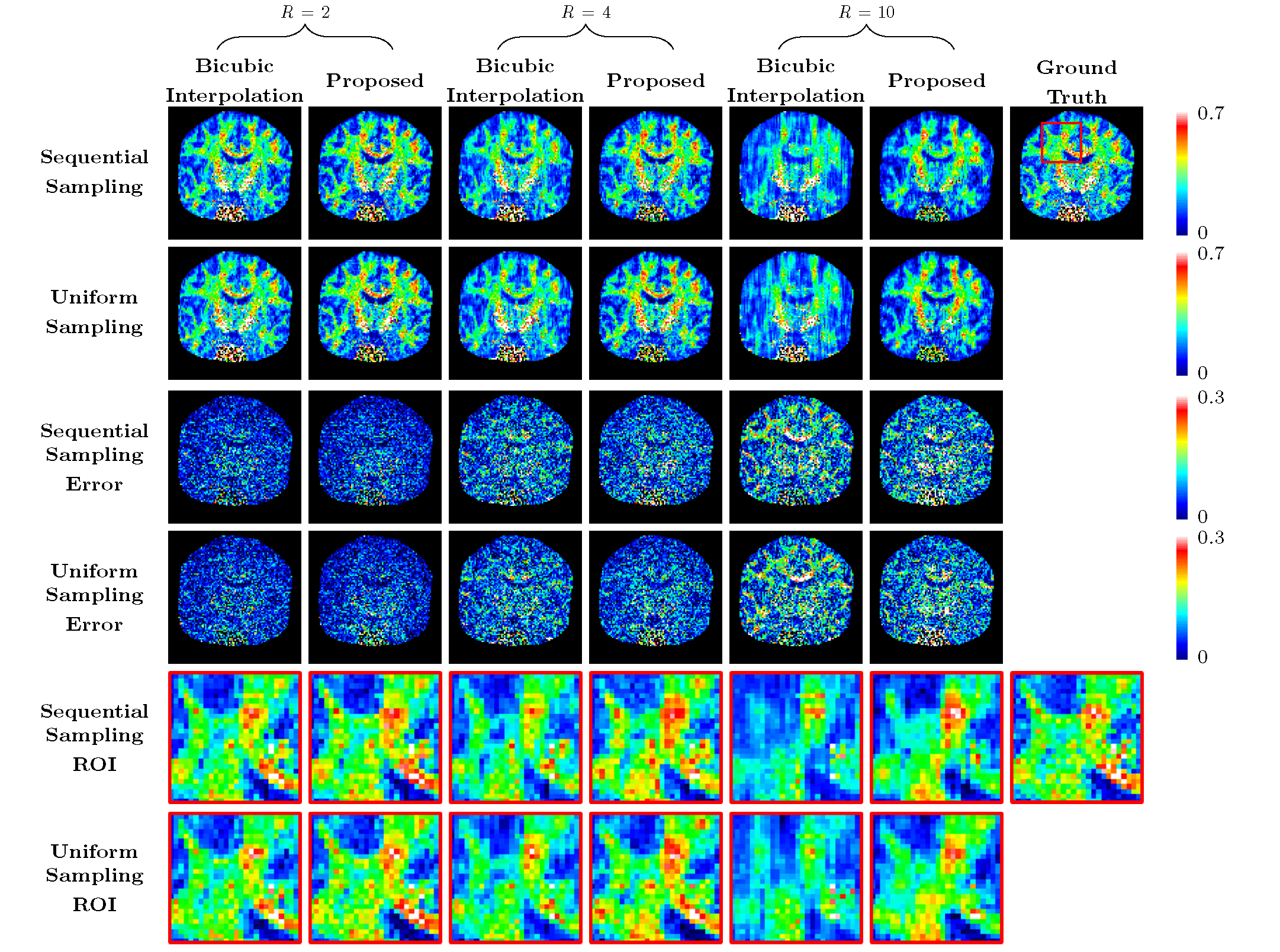
We evaluated our method under various acceleration factors $$$R=2, 4, 10$$$ for $$$b=2000 ~\text{s/mm}^2$$$. For $$$R=2$$$, we selected the 1st to 10th cycles from 20 cycles. For $$$R=4$$$, we selected the 1st, 3rd, 5th, 7th, and 9th cycles. For $$$R=10$$$, we selected the 1st and 16th cycles. Training was carried out using $$$5\times 5\times 1\times 48$$$ input patches and $$$5\times 5\times R\times 48$$$ output patches. The numbers of subjects for training, validation, and testing were 4, 1, and 2, respectively.
We compared our method with bicubic interpolation and 3D U-Net¹ applied to the input upsampled by bicubic interpolation. The quantitative results are summarized in Figure 3. Representative GFA results, shown in Figure 4, indicate that the proposed method recovers more structural details even for high acceleration factors. Note that the input data is not exactly equally-spaced slices. We also compare GFA results with retrospective slice-undersampling for equally-spaced data².
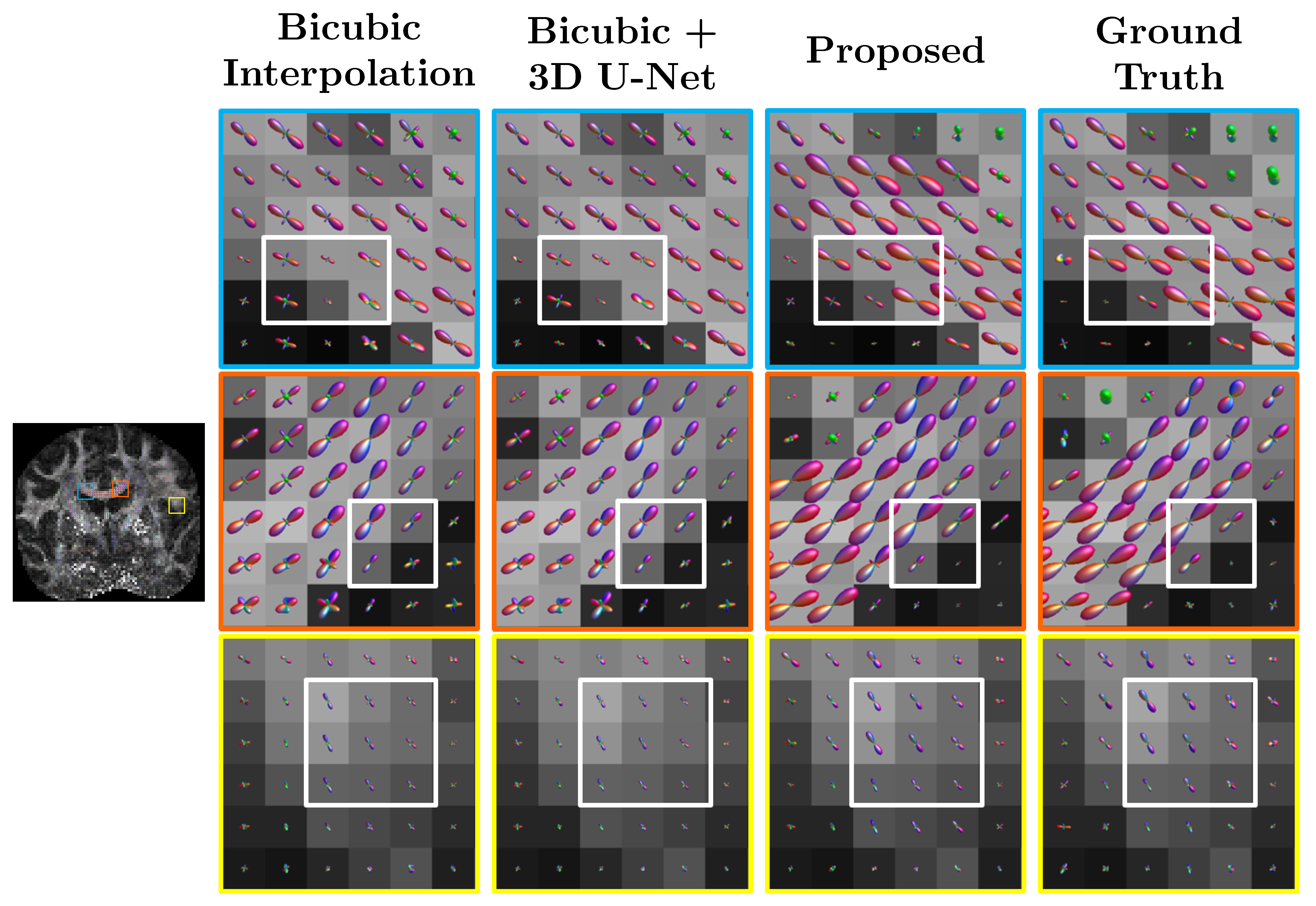
We also generated fiber orientation distribution functions (ODFs) by employing CSD implemented MRtrix3 with the default setting³. Figure 5 shows that our method can yield fiber ODFs that are closer to the ground truth with less partial volume effects.

Conclusion

We have demonstrated that the acquisition of dMRI data can be effectively accelerated by slice-undersampling. Full DW images can be reconstructed via our GCNN, which jointly considers spatio-angular information. Experimental results show that the proposed method can achieve acceleration factor as high as 50 with the help of multiband imaging.

Acknowledgements

This work was supported in part by NIH grants (NS093842, EB006733, and AG060324).