Introduction

The segmentation of human hippocampal subfields on in vivo MRI has gained great interest in the last decade, because these anatomic subregions were found to be highly specialized in recent studies [1-3]. However, manual delineation of hippocampal subregions is extremely labor-intensive and time-consuming, which limits the study to a small sample size. In addition, the inter- and intra- rater reliability is another factor which may influence the statistical power of a study. In this study, we presented a multi-scale Convolutional neural network (CNN) based Automated hippocampal subfield Segmentation Toolbox (CAST) for automatically segmenting hippocampus and some other subregions in medial temporal lobe, which can segment a new subject in one minute.

Methods

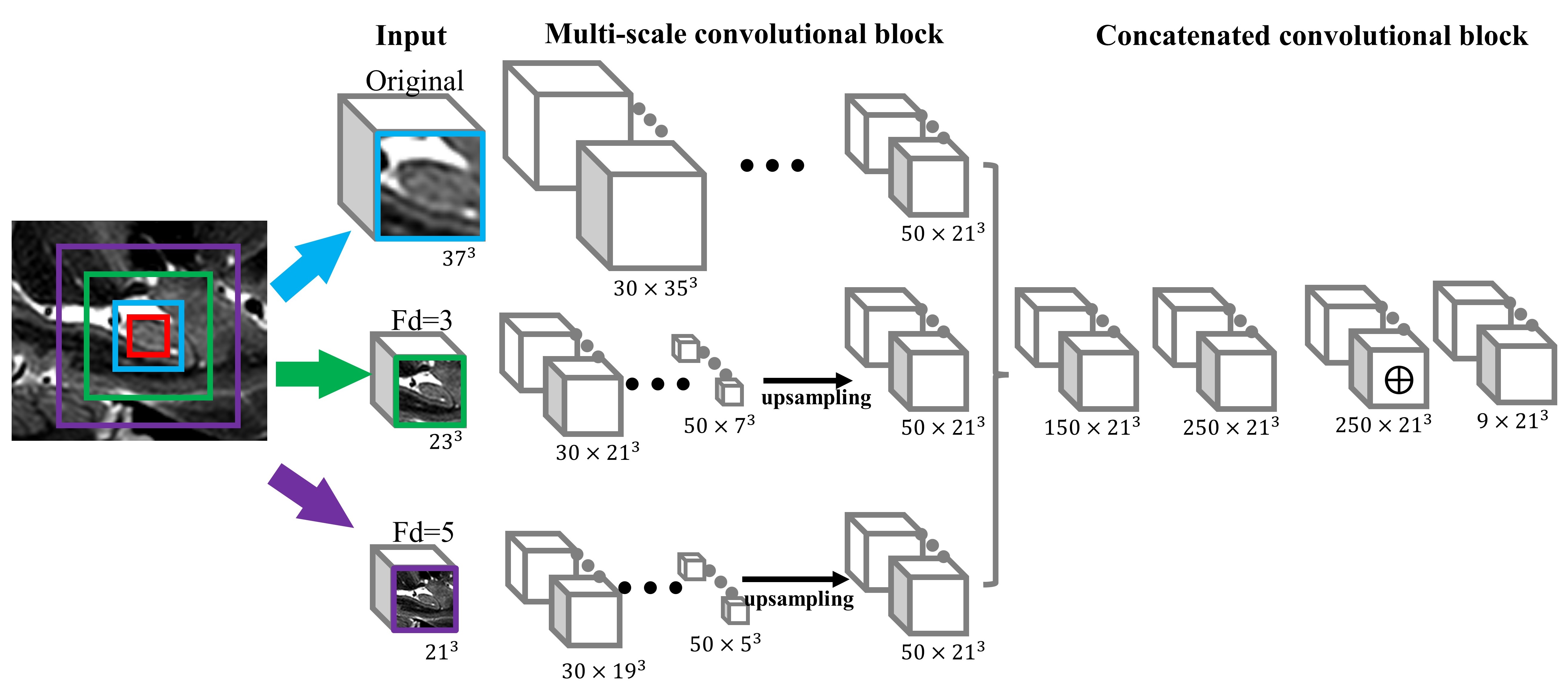
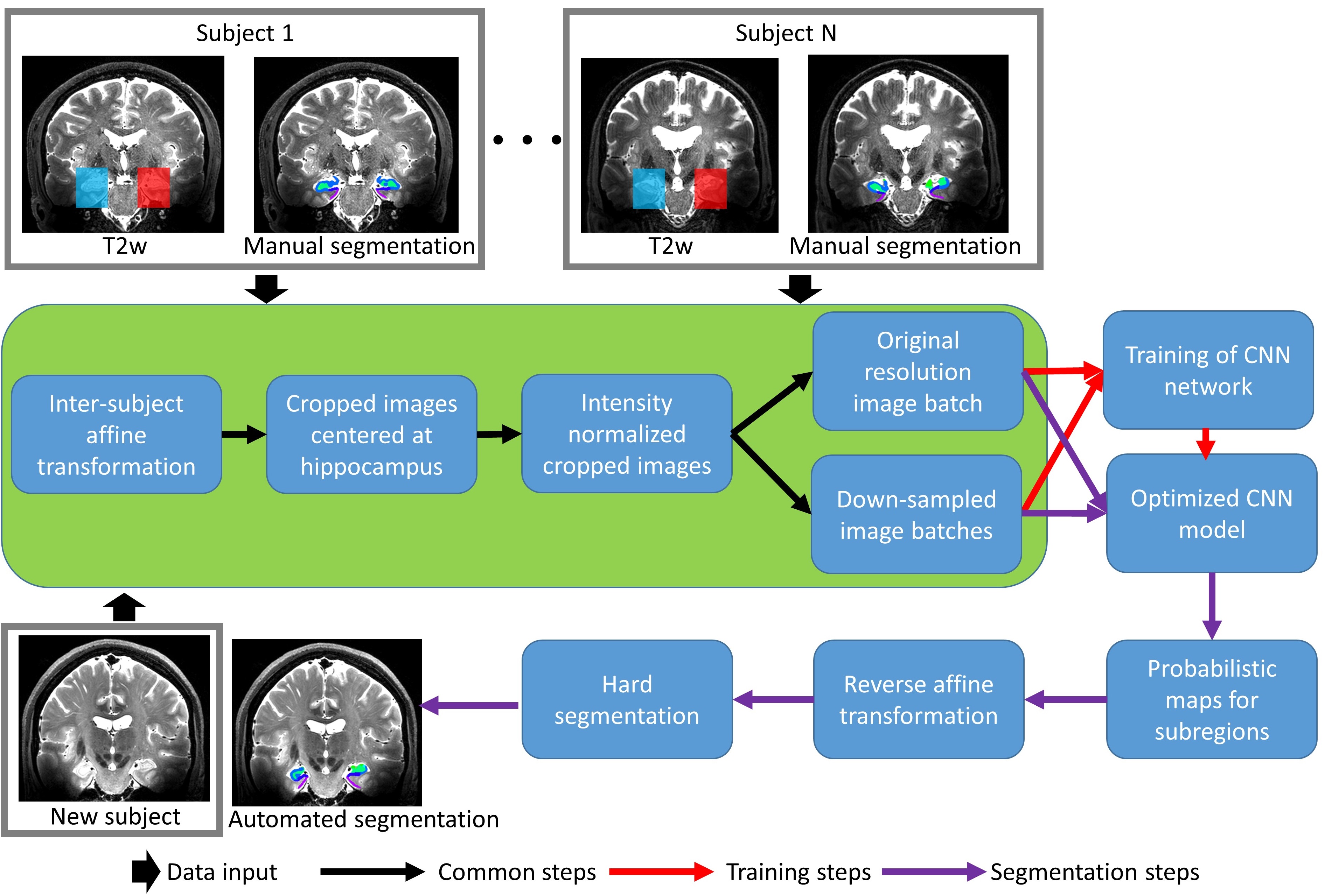
Datasets: CAST segmentation method was applied on a 7T imaging datasets downloaded from ASHS data depository (https://www.nitrc.org/projects/ashs). The 3D T2-weight TSE images from 26 subjects [4], named as UMC dataset, were collected on a 7T Philips MR imaging scanner with 0.7 x 0.7 x 0.7 mm³ isotropic voxel size and interpolated to spatial resolution of 0.35 x 0.35 x 0.35 isotropic voxel size by zero-filling during reconstruction. The manual delineation of hippocampal subregions was performed by the corresponding investigators. Network architecture in CAST: The CNN network as shown in Fig.1 has the original resolution image (blue) and two down-sampled images with factor of 3 and 5 (green and purple, respectively) as input. The green and purple boxes indicate the size of down-sampled images in the original resolution and the input cropped images have the dimension of 37³, 23³ and 21³. These three images are fed to three separate pathways with the same network architecture but independent parameters. Each pathway consists of eight consequential convolutional layers with filter size as 33 and the number of filters as 30, 30, 40, 40, 40, 40, 50 and 50 in the order. Residual connection is implemented for 4th, 6th, and 8th layers to overcome the vanishing gradient problem in a deeper neural network. The two down-sampled pathways are up-sampled to match the dimension of the output from the original pathway and concatenated with dimension of 150 x 21³ for the following concatenated convolutional block. This multi-scale CNN network consists of about 2 million parameters and is developed based on TensorFlow package (https://www.tensorflow.org) and DeepMedic project (https://github.com/deepmedic/deepmedic) [5]. TensorFlow is an open source platform for machine learning, particularly deep learning. DeepMedic provides a general framework for multi-scale convolutional neural network. The training and segmentation pipeline is shown in Fig.2. It takes about three days to train a model on a personal desktop with a Tesla K40c GPU card and less than one minute to segment a new subject with an optimized model. The dice similarity coefficient (DSC) was calculated for each subfield separately and a generalized DSC score was also computed with all subfields considered jointly. The reliability of automated segmentation was measured by using intraclass correlation coefficient (ICC), which measures the absolute agreement under a two-way random effects from a single measurement.

Results

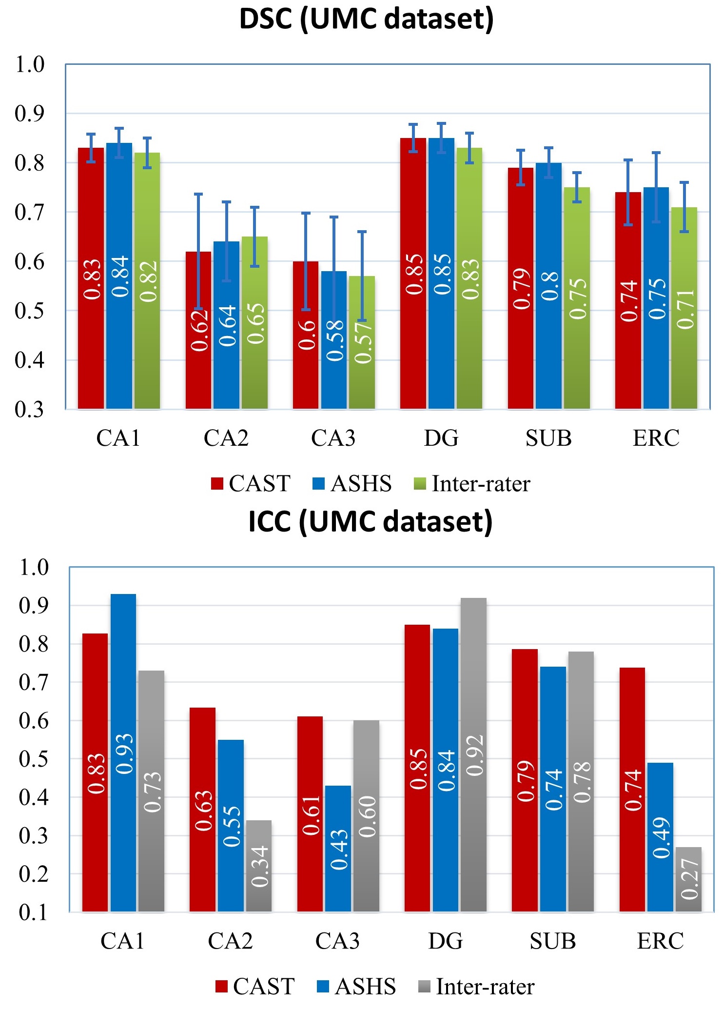
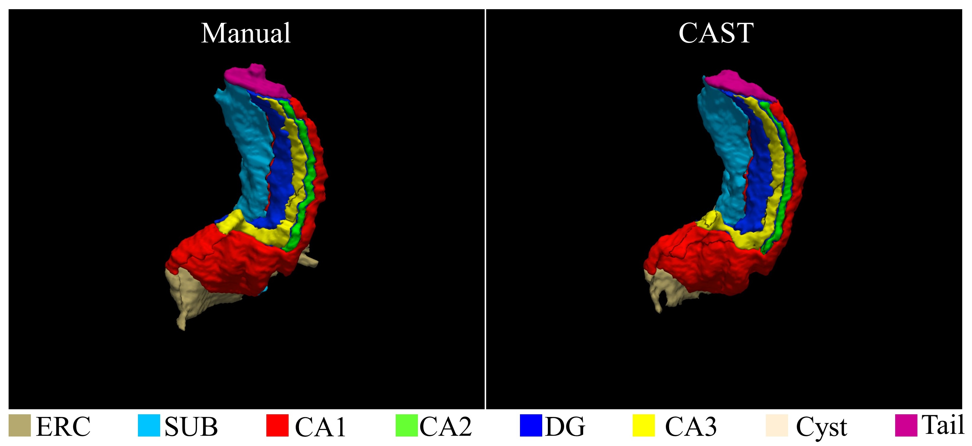
By running CAST with a leave-one-out technique, the DSC and ICC coefficient for the 26 subjects in UMC dataset is shown in Fig.3. Surprisingly, for both CAST and ASHS, the mean generalized DSC across all subfields is 0.80 ± 0.03. Compared to ASHS segmentation, CAST substantially improved the ICC coefficients for CA2, CA3, SUB and ERC by 15%, 42%, 7% and 51%, respectively. However, CAST had worse ICC coefficient for CA1 compared to ASHS by 11%. The 3D rendering plot of CAST and manual segmentations of a single subject with generalized DSC as 0.80 is shown in Fig.4.

Discussion

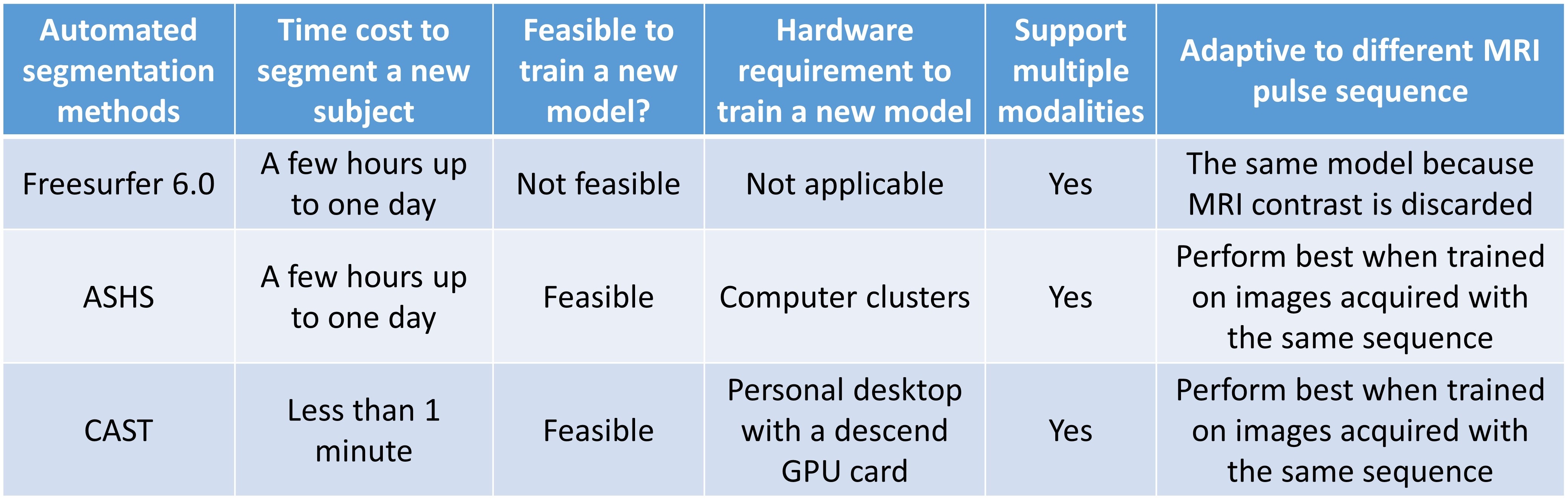
Although the segmentation method in Freesurfer 6.0 is not applied on the dataset because of distinct manual segmentation protocol, a summary of the comparison between Freesurfer 6.0, ASHS and CAST is listed in Table.1. When CAST is applied on a subject with an optimized model, this toolbox only requires raw image as input and can output the segmented images in less than one minute. The computation-efficiency makes CAST applicable for large sample size and instantaneous segmentation. While the same as ASHS that best segmentation is achieved with a customized population specific atlas from the same magnet, CAST can easily be trained on a personal desktop, instead of a computer cluster, to generate the corresponding segmentation model. The automated segmentation overall is very similar to the manual segmentation but with small localized differences observed at the boundary among subfields or between subfields and background. To further investigate the distinct ICC values for CA1 subfield, we have visually inspected the manual segmentations and observed the boundary between CA1 and SUB was defined varying across subjects. Because CAST is designed to learn a consistent rule and apply it to all subjects, the variation within manual segmentation might be related to the inferior performance of segmenting CA1 subfield.

Conclusion

In this study, we present a fast automated hippocampal subfield segmentation method based on a multi-scale deep convolutional neural network, which can segment a new subject in one minute. Compared to current state-of-art method, this method achieves comparable accuracy in terms of dice coefficient and is more reliable in terms of intraclass correlation coefficient for most of subfields.

Acknowledgements

This research project was supported by the NIH (grant 1R01EB014284 and COBRE grant 5P20GM109025), Young Investigator award from Cleveland Clinic, a private grant from Peter and Angela Dal Pezzo, a private grant from Lynn and William Weidner, and a private grant from Stacie and Chuck Matthewson. The atlas and datasets for this project were generously shared by corresponding investigators and publicly available on ASHS data depository.