4261

Design optimization of unshielded 8Tx transmit arrays for the head consisting of loops or dipoles at 7 Tesla

Carel Costijn van Leeuwen¹, Cornelis A.T. van den Berg¹, Dennis Klomp¹, and Alexander J.E. Raaijmakers^1,2
¹Department of radiology, University Medical Center Utrecht, Utrecht, Netherlands, ²Eindhoven University of Technology, Eindhoven, Netherlands

Synopsis

Typical transmit arrays for the head use dipole or loop antennas within an RF shield. However, for certain applications an unshielded head coil array is required. This study explores different designs for unshielded head coil arrays using simulations. Using L-curves, the tradeoff which exists between power efficiency, homogeneity and SAR is evaluated for arrays consisting of loops and dipoles of various dimensions. Loops are found to be superior to dipoles. Small loops yield the highest power efficiency, while larger loops improve homogeneity and SAR efficiency.

Introduction

At ultrahigh field strengths (≥7T) multi-transmit coil arrays are employed to improve transmit field homogeneity. For the head, these arrays typically consist of eight dipole and/or loop antennas within an RF shield. For X-nuclei frequencies at 7T a birdcage body coil is used because of superior B₁ transmit efficiency and homogeneity. To facilitate imaging or spectroscopy of X-nuclei in the head while simultaneously obtaining proton images requires an unshielded ¹H head coil array. This study uses FDTD simulations to compare unshielded eight-channel dipole and loop arrays of different dimensions in terms of transmit efficiency, SAR efficiency and homogeneity.

Methods

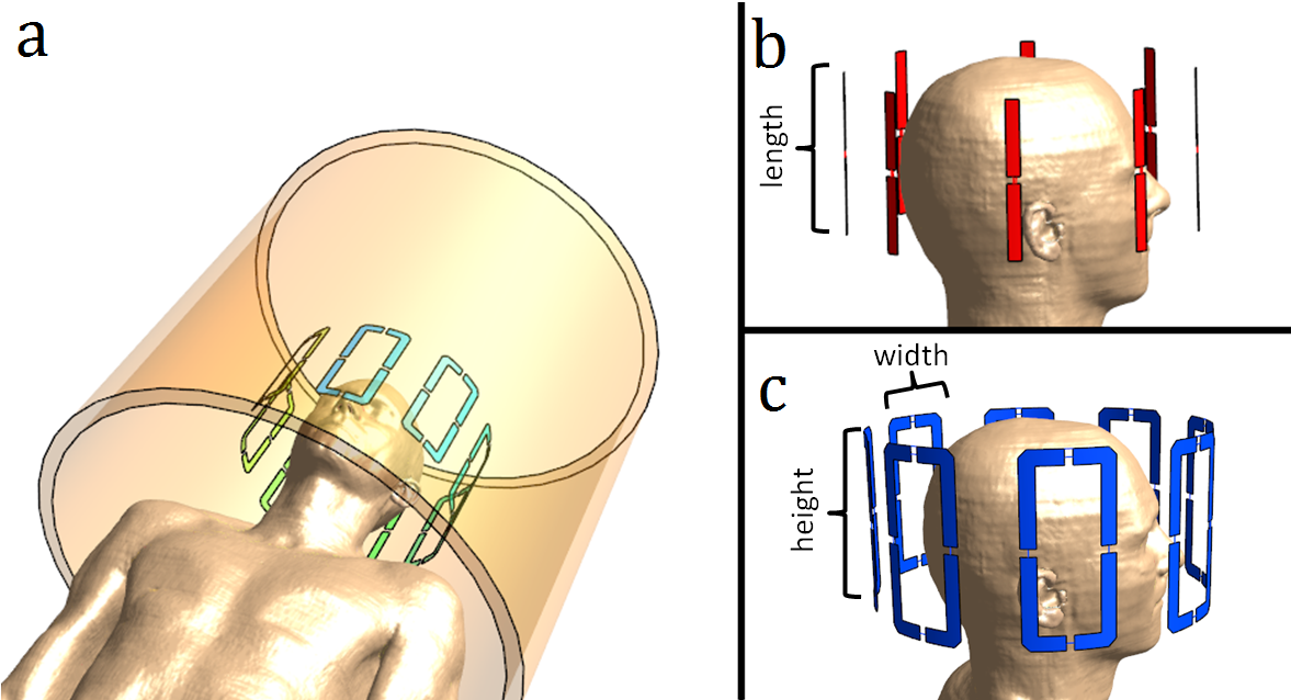
A total of 26 coil array designs are evaluated. 6 Designs consist of dipoles with lengths ranging from 10 to 30 cm. 20 Designs consist of loop coils, with widths and heights varying from 6 cm to 22 cm (figure 1). Each coil array design is simulated using Sim4Life (Zurich MedTech, Switzerland) on the same grid containing 5.9 million cells, using a realistic human model(“Duke”, ITIS foundation¹). Tuning and matching are performed using network co-simulation^2,3. Drive vectors a are obtained by numerical minimization: a = arg_a min{ NRMSE + λ P_forward } where NRMSE denotes the normalised root mean square error with respect to a target B₁ of 1 μT in a mask containing the whole cortex, P_forward = a*a and λ denotes the Tikhonov parameter⁴. Varying λ from 0.0001 to 0.05 yields a set of drive vectors and field distributions, each with a corresponding value for the NRMSE and forward power required. Plotting the NRMSE versus forward power for each drive vector results in an L-shaped curve. For each drive vector peak SAR_10g and accepted power are computed. This allows us to evaluate the tradeoff between homogeneity, SAR and accepted or forward power.

Results

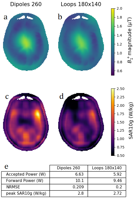
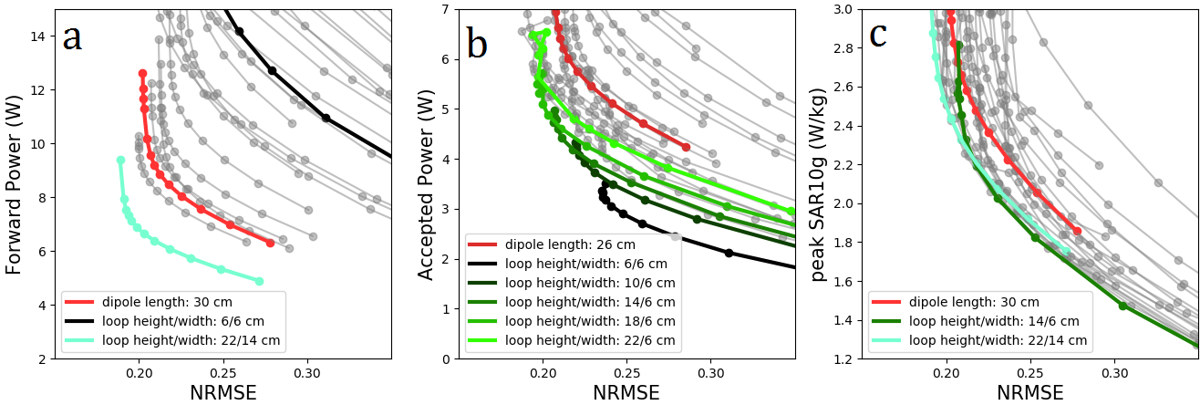
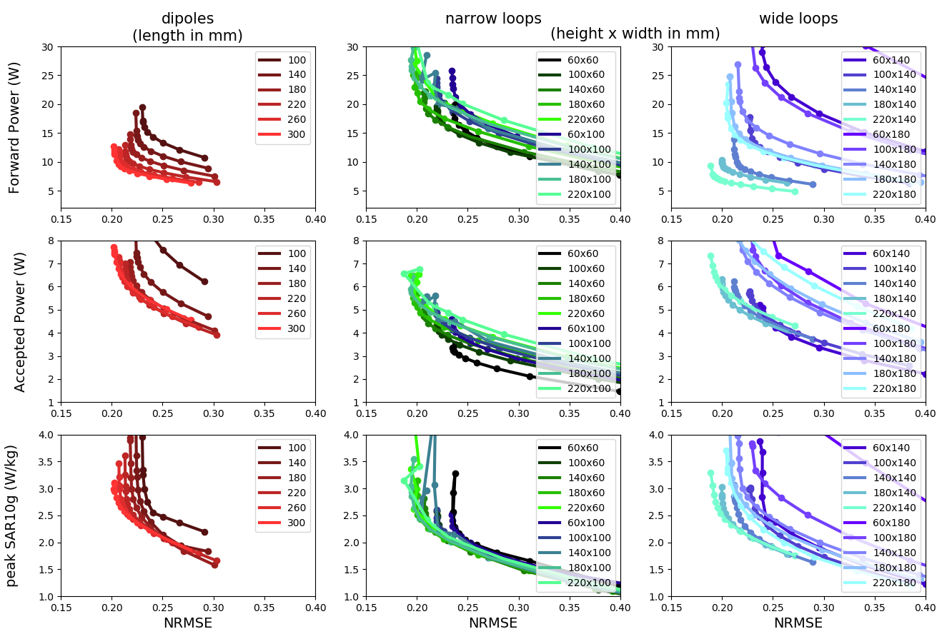
Figure 2 shows two typical examples of field distributions and corresponding metrics which resulted from the minimization process. Figure 3 shows the L-curves of all investigated designs in anonymous grey with a selection of designs highlighted in color. Three types of L-curves are presented: NRMSE versus forward power, accepted power and peak SAR. For the sake of completeness, figure 4 shows every L-curve with model dimensions labeled. In terms of forward power, the best performing models are loop arrays with a width of 14 cm. This is the width dimension where the overlap between neighbouring loops is close to 10% of their surface area, which reduces coupling. In terms of accepted power the narrow loops perform best. The highlighted results in figure 3b show that the smallest loops are most efficient, at the cost of homogeneity. As loop height increases, the arrays are able to produce more homogeneous fields, at the cost of increased power requirements. In terms of SAR the tall loop coils perform best. Of the tall loops, the narrow ones perform slightly better at low SAR and high NRMSE, while the wide ones perform slightly better at high SAR and low NRMSE.

Discussion

With respect to maximizing power efficiency, reduction of inter-element coupling is very important. This study effectively only takes into account geometrical decoupling via overlap, while other methods exist, such as inductive decoupling. Many of the arrays which perform well in terms of accepted power and SAR are strongly coupled so must be decoupled in some other way to achieve a properly functioning transmit array. In no situation do dipoles outperform loops, however this study only considers plain dipoles and leaves variants like folded or fractionated dipoles out of scope. Also, combinations of loops and dipoles could prove beneficial. Future studies aim to include other variants of dipole antennas and the effects of various decoupling strategies.

Conclusion

An explorative study was conducted on the design of unshielded transmit coil arrays. Loops coils were found to perform better than dipoles. Smaller loops were found to be more power efficient. Larger loops performed better in terms of homogeneity and SAR.

Acknowledgements

No acknowledgement found.

References

1. Gosselin M C, Neufeld E, Moser H, Huber E, Farcito S, Gerber L, Jedensjö M, Hilber I, Di Gennaro F, Lloyd B, Cherubini E, Szczerba D, Kainz W, Kuster N, Development of a new generation of high-resolution anatomical models for medical device evaluation: the Virtual Population 3.0, Physics in Medicine and Biology, 59(18):5287-5303, 2014.

2. Kozlov M, Turner R, Fast MRI coil analysis based on 3-D electromagnetic and RF circuit co-simulation. J Magn Reson. 2009 Sep;200(1):147-52. doi: 10.1016/j.jmr.2009.06.005.

3. Beqiri, Arian & Hand, Jeff & Hajnal, Joseph & Malik, Shaihan. (2014). Comparison between simulated decoupling regimes for specific absorption rate prediction in parallel transmit MRI. Magnetic Resonance in Medicine. 74. 10.1002/mrm.25504.

4. Grissom, W. , Yip, C. , Zhang, Z. , Stenger, V. A., Fessler, J. A. and Noll, D. C. (2006), Spatial domain method for the design of RF pulses in multicoil parallel excitation. Magn. Reson. Med., 56: 620-629. doi:10.1002/mrm.20978

Figures

Figure 1: (a) Simulation model, depicting Duke¹, the outer shield of the bore and an example set of eight loops. (b) example model with 140 mm long dipoles. (c) example model with loops. height/width = 140 mm/60 mm

Figure 2: Example results from the minimization, for a typical sets of dipoles (a,c) and loops (b,d). In this case the minimization was performed with a λ of 0.0025. Top row (a,b) shows B₁⁺ magnitude, bottom row (c, d) shows 10gram-averaged SAR distributions of a coronal slice, positioned just above the eyes. The table (e) shows additional metrics from these distributions.

Figure 3: L-curves with respect to forward power (a), accepted power(b) and SAR(c). Most arrays are depicted in gray for improved readability, except for some notable examples. In each case the best performing dipole array is depicted in red. Well-performing or otherwise noteworthy loop arrays are also coloured and labeled.

Figure 4: All L-curves. Left, center and right columns contain dipoles, narrow loops and wide loops respectively. Top, middle and bottom row plot NRMSE versus forward power, accepted power and peak SAR10g respectively. The colours are coded as follows: for dipoles: more red = longer. for loops: more blue = wider, more green = taller.

Proc. Intl. Soc. Mag. Reson. Med. 28 (2020)

4261