4244
Gradient design for a low-field Halbach array using the Target Field Method
Patrick Fuchs1, Bart de Vos1, Thomas O'Reilly2, Andrew Webb2, and Rob Remis1
1Circuits and Systems, Delft University of Technology, Delft, Netherlands, 2C.J. Gorter Center for High Field MRI, Leiden University Medical Center, Leiden, Netherlands
1Circuits and Systems, Delft University of Technology, Delft, Netherlands, 2C.J. Gorter Center for High Field MRI, Leiden University Medical Center, Leiden, Netherlands
Synopsis
We describe the application of the target field method for designing three-axes gradients for the transverse magnetic field produced by a Halbach array, as well as verify this method by constructing a set of 3 gradient coils and using it for 3D imaging. Additionally an open-source tool is described which allows for easy gradient design using this method.
Introduction
The need for MRI scanners in a low resource setting is becoming more apparent and is starting to receive more attention in the MR community. One promising, low cost, approach to generating magnetic fields suitable for MRI in these low resource settings is using permanent magnets arranged in a Halbach configuration. The B0 field produced by such a configuration is transversely oriented to the bore, orthogonal to most clinical systems where the field is produced along the bore of the system.One common and powerful approach to the target field method initially proposed by Turner [1]. In this current work the method was adapted to generate gradient coils for systems where the B0 field is oriented across the bore. The method is then used to design a set of gradient coils for a 50 mT homogeneity-optimised Halbach array with a 27 cm bore diameter [2]. After validating the design method the tools used to compute the gradient current paths have been integrated into an easy to use open-source tool.
Method
The different orientation of the magnetic field relative to the Z axis changes the relationship between the magnetic field and magnetic potential so that $$$\tilde{B}_{x}=-\partial_r \tilde{\Phi}\cos(\phi)+\frac{jm}{r}\tilde{\Phi}\sin(\phi)$$$ as opposed to $$$\tilde{B}_{z}=-jk\tilde{\Phi}$$$ for the original target field method. This adaptation gives the following expressions for the $$$\phi$$$ component of the current densities:$$J^x_{s:\phi}=-j\frac{bg_x}{{\pi}a\mu_0}\cos{(2\phi)}\int_{k=-\infty}^{\infty}\frac{\tilde{\Gamma}_{xy}(k)\tilde{T}(k)}{\frac{|k|}{k}K_{2}'(|k|a)\left[|k|I_{2}'(|k|b)+\frac{2}{b}I_{2}(|k|b)\right]}e^{jkz}\text{d}k$$
$$J^y_{s:\phi}=-j\frac{bg_y}{{\pi}a\mu_0}\sin{(2\phi)}\int_{k=-\infty}^{\infty}\frac{\tilde{\Gamma}_{xy}(k)\tilde{T}(k)}{\frac{|k|}{k}K_{2}'(|k|a)\left[|k|I_{2}'(|k|b)+\frac{2}{b}I_{2}(|k|b)\right]}e^{jkz}\text{d}k$$
$$J^z_{s:\phi}=-j\frac{g_z}{{\pi}a\mu_0}\cos{(\phi)}\int_{k=-\infty}^{\infty}\frac{\tilde{\Gamma}_z(k)\tilde{T}(k)}{\frac{|k|}{k}K_{1}'(|k|a)\left[|k|I_{1}'(|k|b)+\frac{1}{b}I_{1}(|k|b)\right]}e^{jkz}\text{d}k$$
with $$$\tilde{\Gamma}_{xy}(z,d)=\frac{1}{1+(z/d)^n}$$$ and $$$\tilde{\Gamma}_{z}(z,d)=\frac{z}{1+(z/d)^n}$$$ the gradient shape functions for the X/Y gradients and Z gradient respectively, $$$\tilde{T}(k)=e^{-2(kh)^{2}}$$$ the apodisation term used for regularisation $$$I$$$ and $$$K$$$ the modified bessel function of the 1st and 2nd kind with the prime indicating differentiation with respect to the argument, a the radius of the gradient cylinder, b the radius of the cylinder on which the target field is prescribed, d the targeted linear region and $$$g_{\alpha}$$$ the targeted gradient strength.
The current paths were computed using Matlab and consequently exported to a magnetostatic solver in the CST software suite (Dassault Systemes, Vélizy-Villacoublay, France) to verify the field produced by the gradient coils. The field error is defined as $$$\epsilon(x,y)=\frac{\left|B_{x}(x,y)-B_{x}^{ideal}(x,y)\right|}{\left|B_{x}^{ideal}(x,y)\right|}$$$. A set of X, Y and Z gradients with a length and diameter of 35 cm and 270 mm, 274 and 278 mm respectively were designed for optimal linearity over a 20 cm spherical volume and subsequently constructed using 1.5 mm diameter copper wire pressed in to 3D printed moulds fixated on a plexiglass cylinder. The Y and Z gradients were constructed with 12 windings in each quadrant, the X gradient was designed with 15 windings in each quadrant. The gradient field of each coil was mapped through the isocentre of the magnet using a Hall probe attached to a 3D positioning system [3]. Images of a galia melon were acquired using a 3D turbo spin echo sequence with the following parameters: FoV: 192 x 192 x 192 mm, acquisition matrix: 128 x 128 x 128, TR/TE: 3000 ms/20 ms, acquisition bandwidth: 20 kHz, echo train length: 64, no signal averaging, acquisition time: 12 minutes 48 seconds.
Results
Wire patterns for the three gradient generated gradient coils are shown in figure 1, note that the Y and Z gradients are identical but shifted 45 degrees with respect to each other. Figure 2 shows the deviation from linearity of the three gradient coils which shows the expected lower linearity of the X gradient compared to the Y and Z gradients that is intrinsic to the B0 field orientation. Measured gradient profiles for the three gradient coils shown in figure 3. Measured gradient efficiency for the X, Y and Z gradients are 0.52, 0.95 and 1.02 mT/m/A respectively. The inductance of the constructed X gradient was 180 µH, and 225 µH for the Y and Z gradient coils, the resistance for all 3 coils was 0.4 Ohms. Figure 4 shows turbo-spin echo images acquired of a melon with no corrections for gradient non-linearity performed. An open-source tool has been written in Python 3.7 to generate the gradient coils and simulate the fields generated by the coils and can be downloaded at https://github.com/LUMC-LowFieldMRI/GradientDesignTool. A screenshot is shown in Figure 5.
Discussion
The target field method has been adapted to produce gradient coils suitable for magnets where the B0 field is oriented across the bore. The method provides a rapid calculation of the surface currents, and ultimately the wire pattern, required to generate a target magnetic field. The speed of the computation means that parameter sweeps to optimise a particular attribute of the gradient coils can be performed quickly. There is excellent agreement between the simulated and generated gradient fields and the linearity of the Y and Z gradient is very high. The X gradient proves to be a challenging geometry but distortions introduced by gradient non-linearity can be corrected for in post-processing as is also done on commercial scanner. An open-source graphical tool has been created and is shared online, which provides an easy to use interface for studying coil performance and facilitates construction of the gradient coils by exporting the wire patterns to a CAD friendly format.Acknowledgements
This work is supported by the following grants:Horizon 2020 ERC FET-OPEN 737180 Histo MRI, Horizon 2020 ERC Advanced NOMA-MRI 670629, Simon Stevin Meester Award and NWO WOTRO Joint SDG Research Programme W 07.303.101.References
[1] R Turner “A target field approach to optimal coil design”, J. Phys. D, 19(8), 1986
[2] T O’Reilly et al. “Three-dimensional MRI in a homogenous 27 cm diameter bore Halbach array magnet”, J Magn Reson, 307:106578, 2019
[3] Han H et al. “Open Source 3D Multipurpose Measurement System with Submillimetre Fidelity and First Application in Magnetic Resonance”, Sci. Rep, 7:13452, 2017
Figures
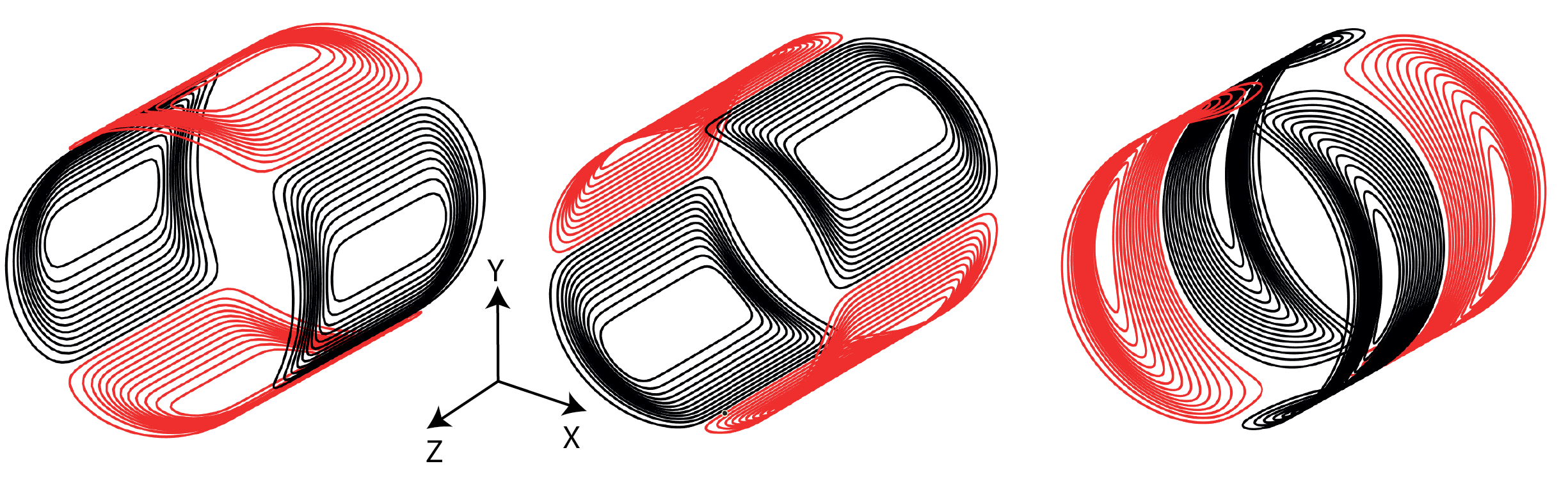
Left)
X, middle) Y, Right) Z gradient coils designed using a target field method
adapted for Halbach arrays where the B0 field is oriented in the X direction.
The colour of the wires indicate opposite current directions.
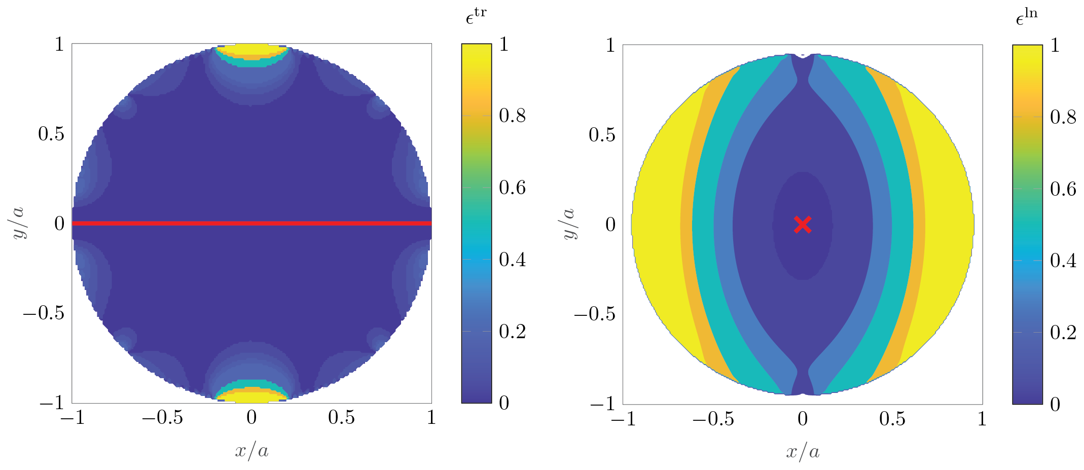
Deviation from linearity of the gradient
field of the left) Y and Z, right) X gradient coils: the red line and cross show
the direction of the gradients relative to the plot. The Y and Z gradients have
a linearity error of less than 5% over 70% of the diameter of the bore, the X gradient
has an error of less than 5% over 20% of the diameter of the bore. Increased
non-linearity is expected for the X gradient as the B0 field is oriented across
the bore of the magnet.
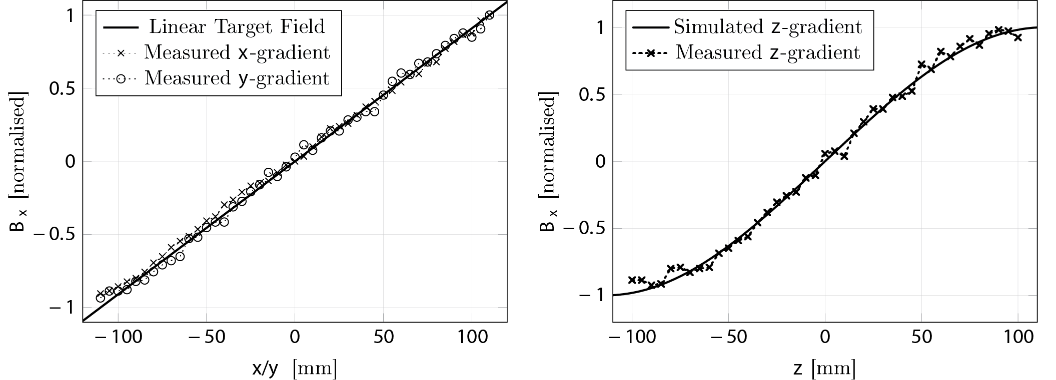
Simulated
and measured gradient field strengths of the three gradient coils.
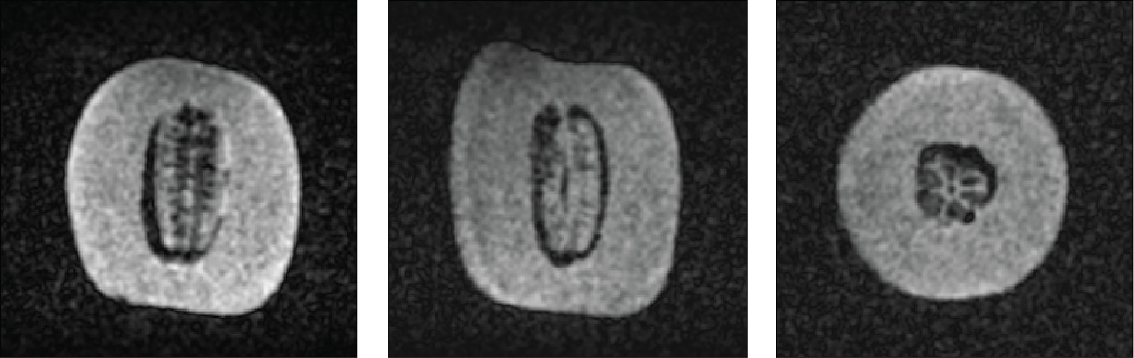
Images
acquired in a 50 mT Halbach array based MRI scanner with a 3D turbo spin-echo sequence
with the following parameters: FoV = 192 x 192 x 192 mm, acquisition matrix =
128 x 128 x 128, TR/TE = 3000 ms/20 ms, acquisition bandwidth = 20 kHz, echo
train length = 64, no signal averaging, acquisition time = 12 minutes 48
seconds.
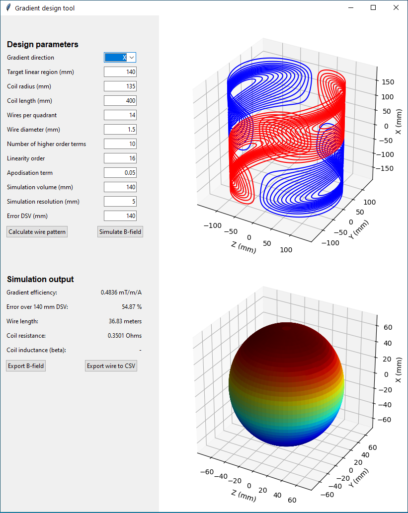
A
screenshot of the gradient design tool developed to allow for easy optimisation
of the relevant parameters. Properties of both the coil itself and the magnetic
field generated by the coil are calculated and the wire patters can be exported
to a CSV file which can be imported in to many computer aided design (CAD)
programs to facilitates easy construction of the gradient coils. The source
code for the tool can be found on Github.