4240
Gradient induced heating of components used in RF coil design1Institute for Biomedical Engineering, ETH Zurich and University of Zurich, Zurich, Switzerland
Synopsis
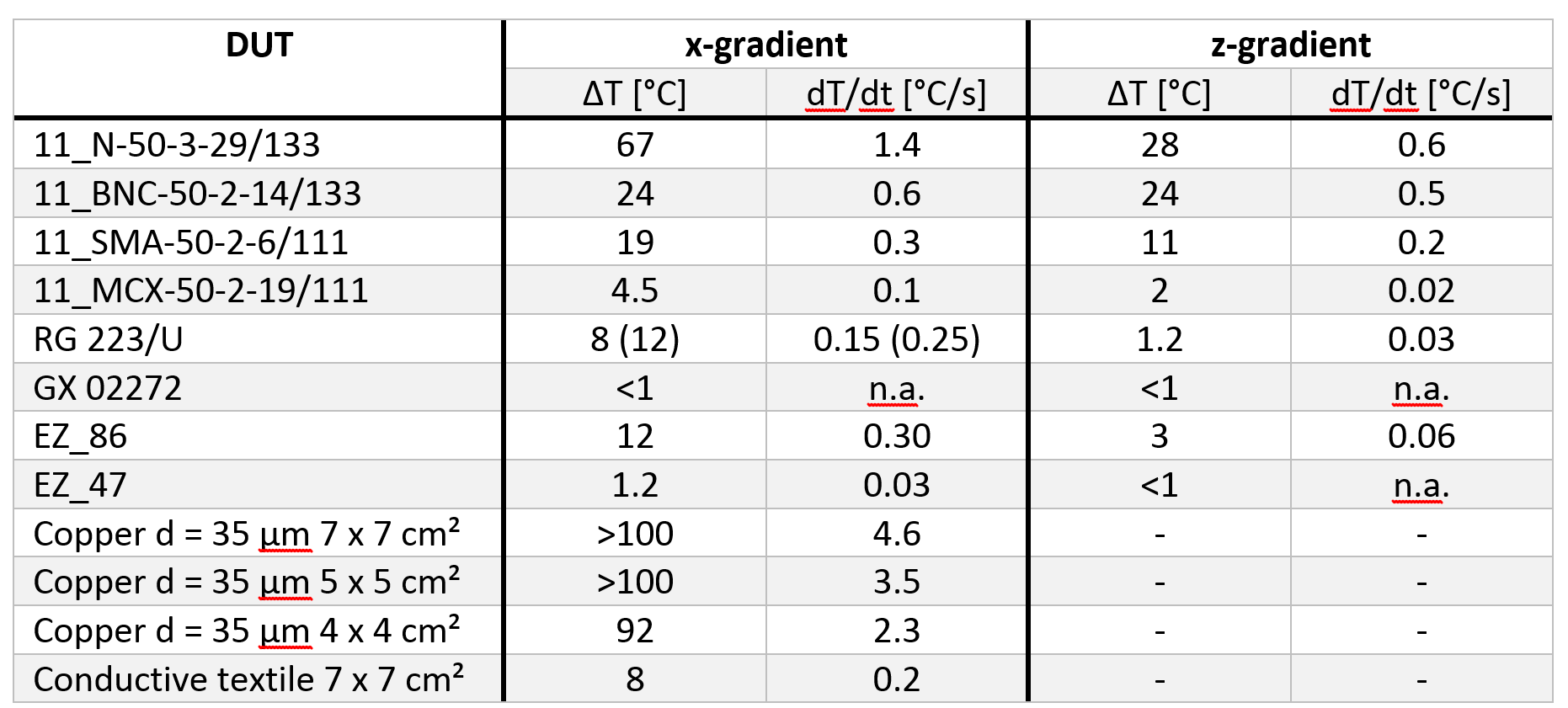
Gradient induced heating is relevant for RF coils used in recent high-performance gradient coils. In this abstract, we investigate the predictability of gradient induced heating on the basis of theoretical gradient field data. Furthermore, the heating of components usually used for coil construction e.g. different plugs, cables and shielding materials under intense gradient usage (EPI readout with 100 mT/m and 1200 mT/m/s at almost 100% duty cycle for 1 min) was measured. Depending on the position and orientation we observe temperature increases up to 67°C for an N-plug and 12°C for a coaxial cable.
Introduction
Since eddy currents scale up with increasing gradient strength and slew rate, gradient induced heating is relevant for conducting structures placed inside e.g. RF coils (1). In this study, we investigate the heating of components commonly used in RF coil construction depending on their position and orientation.Methods
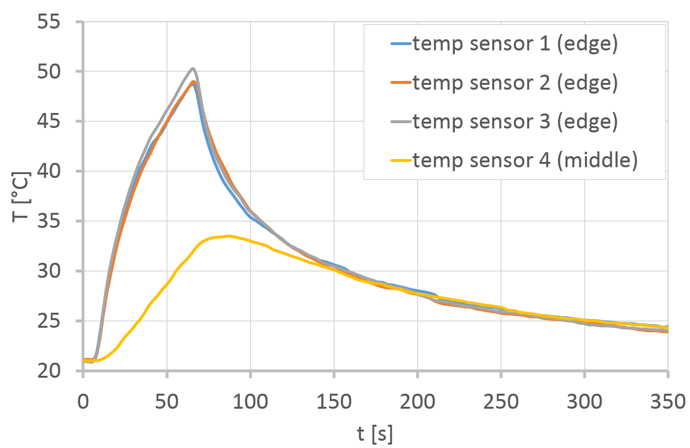
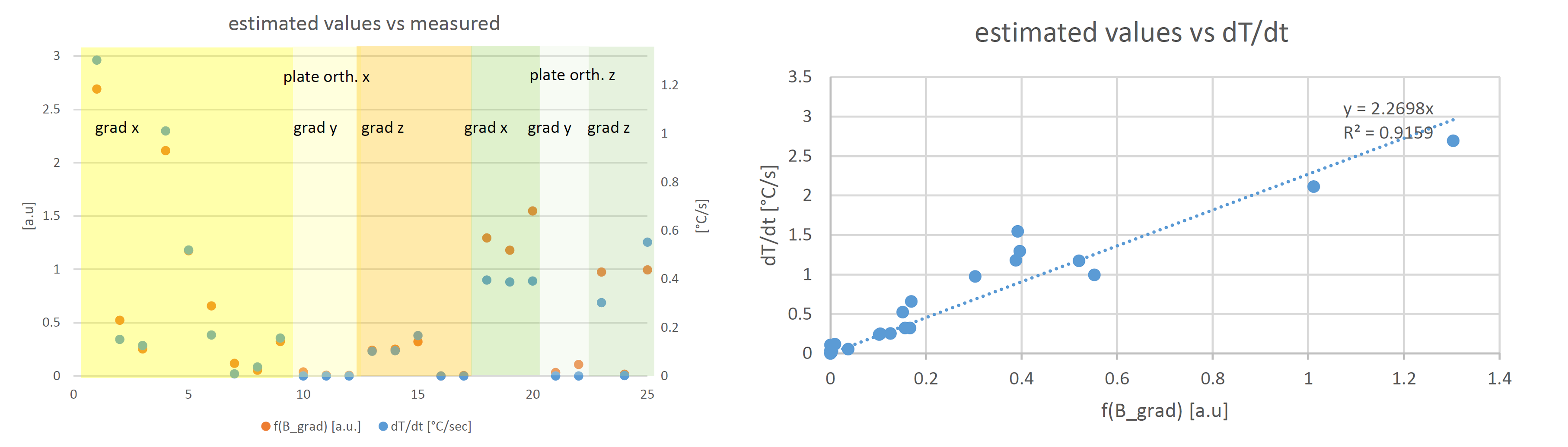
Theoretically, the deposited power causing heating will be proportional to the square of the gradient fields (2,3), if the slew rate has a constant absolute value. For objects with a negligible extension in one dimension, only field components perpendicular to its main surface need to be taken into account. In this work, this relation is described by f(B_grad) and is used to estimate temperature increase.All measurements were performed on a whole body 3 T scanner in combination with a high-performance gradient insert (4). The device under test (DUT) was heated by an EPI readout with almost 100% duty cycle as well as a gradient strength of 100 mT/m, a slew rate of 1200 mT/m/ms and an in-plane resolution chosen to reduce the plateau with constant gradient strength to zero. Meanwhile, the temperature profile was observed with optical temperature sensors (T1C-2M-PP10 + 4 channel reflex fiber optic conditioner, Neoptix, Canada), which were fixed to the DUT with tape. Afterwards, the linear temperature increase (dT/dt) within 4 s at the beginning of the heating period as well as the absolute temperature difference (ΔT) after 1 min heating was evaluated. Measurements above 120°C were interrupted manually.
First, the heating of a FR4 board with a 35 μm thick copper area of 7 x 7 cm² was investigated at different positions and orientations in the gradient tube as well as under different measurement gradient orientations. One temperature sensor was placed in the middle and three others at the edges of the copper area.
Afterwards, this experiment was repeated for other DUTs centered at position x = -15 cm, y = 0 cm, z = -17 cm relative to the gradient isocenter:
- FR4 boards with a 35 μm thick copper area of 5 x 5 cm² and 4 x 4 cm²
- A conductive textile (4715-Conductive textile tape with standard adhesive, Holland Shielding, The Netherlands) with an area of 7 x 7 cm²
- Different straight cable RF plugs (HUBER+SUHNER, Switzerland) orientated parallel to the z-axis of the magnet. The temperature sensor was fixed at the shell.
- Different RF cables (HUBER+SUHNER, Switzerland) with a length of 30 cm routed parallel to the z-axis of the magnet. If applicable, the plastic jacket was removed locally to place an additional temperature sensor directly on the metallic shield. Temperature sensors were fixed in the middle of the cable.
Results & Discussion
The typical temperature profiles as shown in Figure 1 indicates, that the size of the copper area is too big to neglect heat transfer. However, the chosen size was a compromise between sensitivity at locations with limited heating and accuracy. Gradient field deviations within the board area were checked to be small, but could be an additional error source.As expected from theory, the proportionality factor (figure 2b) between the measurements and f(B_grad) is independent of gradient axis and sample orientation (figure 2a). Nonetheless, the confidence value is only 0.92, which might have been caused by limitations in positioning, sample size, variations in cooling effects (airflow) and the temperature measurement method itself (fixation and positioning of sensors). Obviously, the linearity factor must be calibrated for every object.
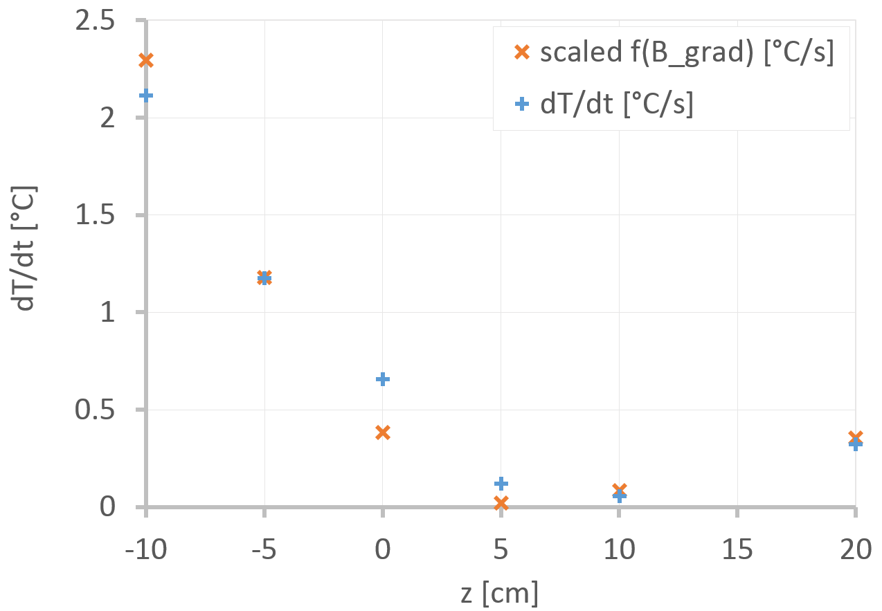
The wanted gradient fields in z-direction used in MRI would only heat the board, if oriented perpendicular to the z-axis. However, for the gradient insert field data indicate highest eddy currents when placed orthogonal to x-axis at x = -15 cm, y = 0 cm, z = -17 cm. Measured data (figure 3) confirms that x and y components of the gradient field, which also lead to known concomitant field, are not negligible.
Larger components and ticker cables heat up faster as summarized in table 1. Reducing the area of conducting structures (e.g. slotting) and conductivity at low frequencies (conductive textile (5)) minimizes the temperature increase.
The slew rate of the insert gradient is 6-times higher than the one of the default gradient system, which would result in 36-times higher power deposition. However, only an approximately 9-times higher initial temperature increase (dT/dt 4.3°C/s vs 0.47°C/s) was observed. This might be explained by the smaller diameter and shorter length in z-direction as well as unknown non-z-components of the standard system.
As demonstrated, temperature measurements could localize structures with strong eddy currents in RF coils and help to reduce image artefacts.
Conclusion
In high-performance gradients eddy current induced heating is significantly increased and may lead to serious problems. It might as well become more relevant for implants.Acknowledgements
No acknowledgement found.References
1. Rösler MB, Weiger M, Brunner DO et al. An eight-channel array coil for zero echo time imaging. In Proceedings of the 27th Annual Meeting of ISMRM, Montreal, QC, Canada 2019. p. 438.
2. Graf H, Steidle G, Schick F. Heating of metallic implants and instruments induced by gradient switching in a 1.5‐Tesla whole‐body unit. Journal of Magnetic Resonance Imaging: An Official Journal of the International Society for Magnetic Resonance in Medicine. 2007;26(5):1328-1333.
3. El Bannan K, Handler W, Chronik B, Salisbury SP. Heating of metallic rods induced by time‐varying gradient fields in MRI. J Magn Reson Imaging. 2013;38(2):411-416.
4. Weiger M, Overweg J, Rösler MB et al. A high-performance gradient insert for rapid and short-T2 imaging at full duty cycle. Magn Reson Med. 2018;79(6):3256-3266.
5. Weiger M, Brunner DO, Schmid T et al. A virtually 1H‐free birdcage coil for zero echo time MRI without background signal. Magn Reson Med. 2017;78(1):399-407.
Figures