4239
Adaptive Deadtime Compensation Control for MRI Gradient Amplifier
Huan Hu1, Juan A Sabate1, and Ruxi Wang2
1GE Global Research, Niskayuna, NY, United States, 2GE Aviation, Dayton, OH, United States
1GE Global Research, Niskayuna, NY, United States, 2GE Aviation, Dayton, OH, United States
Synopsis
MRI gradient amplifier needs to provide current with extremely high fidelity to the commanded values of any arbitrary shape. Therefore, the control requires very accurate compensations of nonlinearities. One of the major sources is the deadtime among the power semiconductor devices. The existing deadtime compensation was to pre-test the specific system with different current commands and summarize a look-up table for use, which required lots of time and effort and cannot be used for different systems. This abstract demonstrates an adaptive deadtime compensation method which works well under different current commands and different systems without additional hardware cost.
Introduction
Magnetic Resonance Imaging (MRI) uses magnetic field gradients to do spatial encoding for imaging. In the MRI system, gradient amplifier is a switching power supply which is composed of power semiconductor devices to provide the gradient field [1]-[3]. To achieve the required performance, MRI gradient amplifier needs to provide current with extremely high fidelity to the commanded values of any arbitrary shape. Therefore, the control requires very accurate compensations of nonlinearities. One of the major sources of the nonlinearity is the deadtime between the top device and the bottom device to avoid shoot-through. Theoretically, the deadtime compensation varies with different current commands and different systems. The existing deadtime compensation was to pre-test the specific system with different current commands and summarize a look-up table for use, which required lots of time and effort and cannot be used for different systems [4]. This abstract demonstrates an adaptive deadtime compensation method which works well under different current commands and different systems without additional hardware cost [5].Adaptive deadtime compensation method
The two H-bridge gradient amplifier topology is shown in Fig.1 [2]. Ideally, the deadtime compensation dtcmp should be equivalent to the deadtime setting dt for a given current sign and should be zero during the zero-crossing zone. Practically, when considering the output capacitance Coss of the power semiconductor device which may cause resonance with the filter inductance, the effective deadtime is no longer a constant value and is highly depending on the bridge current Ibridge. As shown in Fig.2(a) where the current threshold of the deadtime compensation is $$$Ith= \frac {2 \cdot Coss \cdot Vbus}{dt}$$$, dtcmp can be calculated based on real time operation of the bridges with the accurate Ibridge value (case1: $$$dt_{cmp}=dt$$$ ; case2: $$$dt_{cmp}= \frac{Coss \cdot Vbus}{abs(Ibridge)}$$$ ; case3: $$$dt_{cmp}=dt - \frac{abs(bridge) \cdot dt \cdot dt}{4 \cdot Vbus \cdot Coss}$$$ where Vbus is the DC link voltage). However, it is very challenging to sense the bridge current Ibridge directly due to the high slew rate and high required bandwidth, and it will increase the hardware cost of the MRI system. The existing compensation method was to use the coil current Icoil for approximate Ibridge value and assume a linear change in the compensation during the zero-crossing zone as shown in Fig.2(b). With this method, the compensation for a typical trapezoidal current is shown in Fig. 2(c). Different current slew rates had different slopes and current thresholds Ith, which means a lot of pre-tests should be done to get a relatively accurate look up table and the pre-tests must be repeated to get a new look up table if the system changes such as the filter, deadtime setting or the DC link voltage. To get more accurate compensation, the proposed adaptive deadtime compensation method uses the existing control parameters to calculate the real time ripple and reconstruct bridge current Ibridge_c for deadtime compensation as shown in Fig.2(d). Furthermore, it uses the system information (switching frequency, filter, device information, deadtime setting, etc.) to calculate the accurate deadtime compensation by using the method shown in Fig.2(a), which can fit for any shape of the current commands with different slew rates and amplitudes and can be adjusted easily when the system changes.Gradient Amplifier Simulation and Test Results
To verify the adaptive deadtime compensation method, two cases with different slew rate and amplitude are simulated and compared in PLECS (circuit simulator). Case 1 is 200A peak trapezoidal current command with 0.1A/us slew rate, as shown in Fig.3(a); case 2 is 600A peak trapezoidal current command with 2A/us slew rate, as shown in Fig.3(b). In the middle and bottom figures, the red color represents the waveforms when the existing compensation method with look-up table is used and the blue color represents the waveforms when the adaptive deadtime compensation method is adopted. Apparently, the current error is smaller with the adaptive deadtime compensation in Fig.3(a). Without any changes in the control, the adaptive deadtime compensation can achieve slightly less Ierror as the look-up table method which uses different threshold and slope for this specific current command in Fig.3(b). A full-scale two H-bridge gradient amplifier prototype as shown in Fig.4 has been tested. The preliminary test results for 200A peak with 0.1A/us trapezoidal command are shown in Fig.5, where the purple curve is the coil current Icoil, and the green curve is the current error Ierror. Fig.5(a) shows the current waveforms without deadtime compensation and Fig.5(b) shows the waveforms with the look-up table deadtime compensation method used. As shown in the waveforms, the existing deadtime compensation can help reduce the average current error, but during the zero-crossing zone Ierror is still not small enough due to the inaccurate deadtime compensation. With the adaptive deadtime compensation method, it will help improve the control performance during the zero-crossing zone as well. A comprehensive evaluation driving the different imaging sequences will provide more detailed results for different amplitudes and slew rates.Conclusion
The MRI gradient amplifier requires high current tracking accuracy for the image quality and therefore the compensation of the deadtime impact is critical. The method used in the existing MRI system needs to pre-test the system with all kinds of current command and use the look-up table to optimize the system. With the adaptive deadtime compensation method, it will save lots of effort on the pre-test and is very adaptive for any current command and different MRI gradient amplifier system.Acknowledgements
No acknowledgement found.References
[1] J.Sabate, et al., Proc. IEEE J.Emerg. Sel. Topics Power Electron. 2016. [2] R.Wang. et al., Proc. ISMRM 2018. [3] J.Sabate, et al., Proc. European Power Electronics Conf. 2007. [4] J.Sabate, et al., Proc. IEEE PESC. 2008. [5] H.Hu, et al., Proc. IEEE-Applied Power Electronics Conference 2019.Figures

Fig. 1. Two H-bridge MRI
gradient amplifier
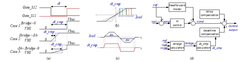
Fig. 2(a) Deadtime
compensation calculation; (b)(c) Existing deadtime compensation method; (d) Proposed
gradient amplifier control architecture
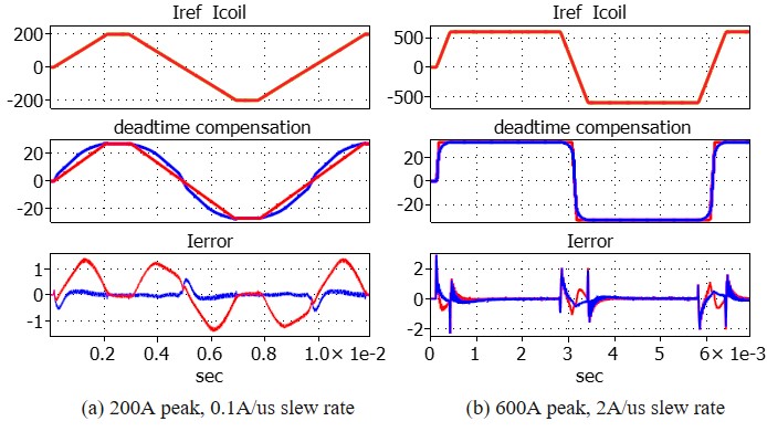
Fig. 3. Simulation
results
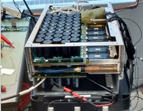
Fig.4. Two H-bridge
MRI gradient amplifier prototype

Fig.5 200A peak,
0.1A/us slew rate trapezoidal test waveforms