4238
Characterization of a permanent magnet based 3D non-linear spatial encoding for ultra-low field MRI1University of Queensland, Centre for Advanced Imaging, Brisbane, Australia, 2Departement of Engineering Physics, FH Muenster University of Applied Sciences, Muenster, Germany
Synopsis
The construction of a permanent magnet based 3D encoding system for an Ultra-Low field MR is presented and its initial characterization is presented. Proposed system moves a single permanent magnet along a prescribed helical path as proposed in our previous numerical study. This initial prototype is built to fit an existing ULF-MRI human extremity system. Preliminary results are in good agreement with the simulations. However, further studies are needed to identify the sources of error and improve the precision of the field estimations towards a practical encoding system.
Introduction
Image generation in conventional MRI systems is achieved by varying the static magnetic field of the scanner linearly in space. The approach allows for fast image reconstruction and equidistant sampling within images. The linearly varying gradient magnetic fields are generated using resistive coils, requiring electric current and can be space consuming,1 making them impractical for portable ultra-low-field (ULF) MRI applications.Previous works have harnessed the intrinsic static field inhomogeneity of a Halbach array for spatial encoding.2 Therein, 2D spatial encoding of the sample was achieved by rotating the Halbach array about the sample and, encoding in the 3rd dimension was realized using RF pulses.3 We previously predicted that 3D images can be generated by moving a single encoding magnet on a linear helical path around a sample (Fig.1).4 We now present the hardware capable of achieving the movement of a permanent magnet over the helical path. Measurements of the encoding fields generated by the prototype are presented and compared with simulation findings.
Methods
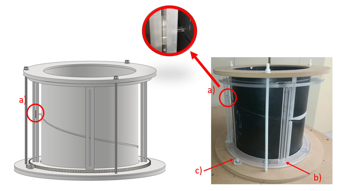
Design and construction of the encoding array: Fig.1 shows the design of the encoding system. The main components include an external acrylic frame that sets the orientation and angular position of the permanent magnet (N48, 25x12x6mm), and an internal concentric HDPE tube (450Øx440L mm) with a helical engraving to set the vertical positioning of the permanent magnet. The frame rotates concentric to the axis of the tube with the aid of a non-metallic bearing array and the tube remains stationary. One frame pillar hosts an encapsulated permanent magnet acting as a vertical rail for the magnet and has a slit for magnet height to be defined by tube's slot through a pin. The slot acts as a sliding rail for the pin, which enforces the permanent magnet to follow the helical path when rotating the frame.Measurements: Magnetic field measurements were confined to the central transverse plane of the cylinder. A single-axis fluxgate magnetometer (Mag-01H, 0.2mT Mag-B probe, Bartington Instruments) was used to map the magnetic flux density. A manually-operated purpose-built magnetometer positioning jig was fabricated (Fig.3A) to map X, Y, and Z field components throughout the field-of-view (120x120 mm) following a horizontal grid of 13x13 points placed at the center of the system. Five encoding positions were evaluated, corresponding to 0°, 90°, 180°, 270° and 360° permanent magnet positions (Fig.3B).
Simulations: COMSOL© simulation results were generated corresponding to the 120x120 mm2 field-of-view of the experimental measurements. The magnetic field produced by the permanent magnet was set to 1.4 T at the center, which corresponds to a class N48 permanent magnet. The location of the permanent magnet in the different experimental setups was measured, and used in the simulations, which allowed us to partially account for manufacturing imperfections.
Data analysis: MATLAB© was used to normalize measured and simulated maps with respect to their corresponding mean values and to perform comparisons. The relative differences between normalized maps where used to generate error maps.
Results
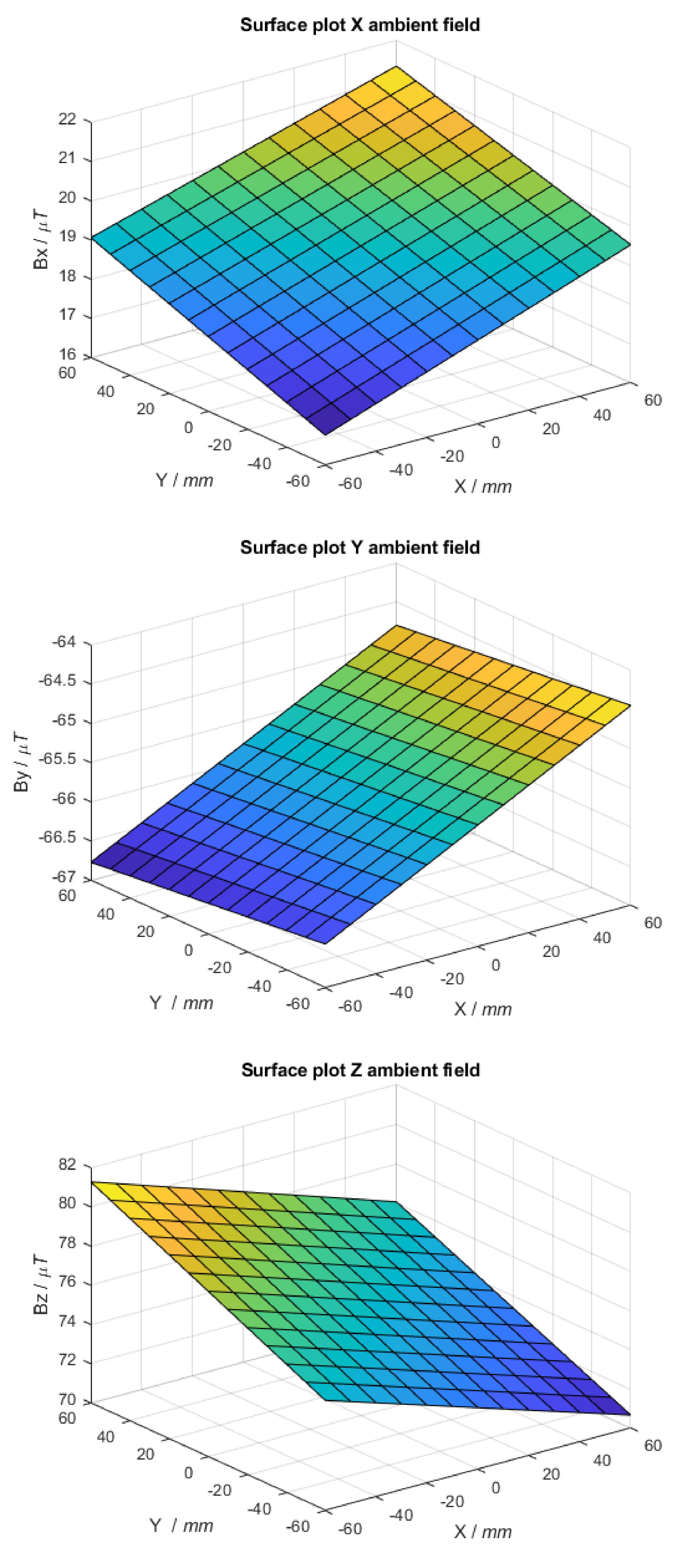
The encoding system constructed ended up with a 565 mm outer diameter, 435 inner diameter and 440 mm height, weight of 5 kg and material costs less than US$1,000. Figure 4 provides the surface plots for the ambient static magnetic fields which were subtracted to obtain the spatial encoding magnetic fields.Measured field maps are shown in Figure 5 corresponding to the 0°, 90°, 180°, 270° and 360° encoding positions. The plots of the difference between measurements and simulations are shown as error plots in Fig.3F-J. The average error was less than 3% in all positions (0° - 2.2%; 90° - 2.7%; 180° - 2.7%; 270° - 2.2%; 360° - 2.8%). Error plots show a level of spatial correlation with increasing field, i.e. errors increase as field strengths increase.
The average value of the experimentally measured magnetic field was on average 7.7% lower than the simulation result.
Discussion
Measurements and simulations were found to be in good agreement. Potential sources for the difference between measurements and simulations include miss-registration between experimental section and simulation slice, and a potentially tilted and non-uniform remanent magnetization of the permanent magnet. These possible issues could be resolved by mapping additional sections and co-registering 3D instead of 2D values, and the characterization of the permanent magnet would additionally help identify error sources.Whilst we assumed the ambient static magnetic field can be interpolated linearly (note we did four corner and one center measurement – Fig.4), non-linear spatial variations between measured points could exist in practice. We expect the non-linear effect to be negligible as the interpolated field maps passed through the measured center point.
The time varying ambient field can also be a source of error as the measurements were taken over two consecutive days. This effect could be mitigated by placing the system in a high permeability shielded room, or by making concurrent ambient field measurements.
Conclusions
Our preliminary non-linear spatial encoding permanent magnet experiment showed good agreement between measurements and simulation. The advantage of our setup is that it is compact, lightweight, inexpensive and requires very low energy consumption. All of these features increase the potential portability of ULF-MRI systems. Additional characterization will help identify the sources of error and improve the precision of field estimations.Acknowledgements
No acknowledgement found.References
1. Sharp, J. C. & King, S. B. MRI using radiofrequency magnetic field phase gradients. Magnetic resonance in medicine 63, 151-161 (2010)
2. Cooley, C. Z. et al. Two‐dimensional imaging in a lightweight portable MRI scanner without gradient coils. Magnetic resonance in medicine 73, 872-883 (2015)
3. Cooley, C. Z., Stockmann, J. P., Sarracanie, M., Rosen, M. S. & Wald, L. L. in Intl Soc Mag Res Med. 4192.
4. Vogel, M.W., Guridi, R.P., Su, J. et al. 3D-Spatial encoding with permanent magnets for ultra-low field magnetic resonance imaging. Sci Rep 9, 1522 (2019)
Figures