Introduction and Purpose

Gradient array systems have been used to generate dynamically controllable magnetic field profiles^1-4. In these systems, multiple gradient coils are driven individually by independent gradient power amplifiers (GPAs). The accuracy of gradient current waveforms has a significant effect on the image quality and providing gradient coil currents with high fidelity might be challenging due to mutual coupling between coils, GPA imperfections, and time-varying parameters in gradient hardware. Although considering the first-order model in the feedforward including mutual coupling provides adequate currents to the coils¹, residual errors due to measurement errors in the determination of model parameters, not considering GPAs in the model, high order effects and time-varying parameters can still decrease the accuracy of coil currents time-courses. A close-loop feedback can be used to overcome these imperfections⁵. In this work, a digital real-time (proportional–integral–derivative) PID controller is designed to compensate for the above-mentioned effects which are not corrected by the feedforward model. The controller also degrades current waveforms sensitivity to the time-varying parameters and undesired external disturbances like droop in the supply voltage.

Methods

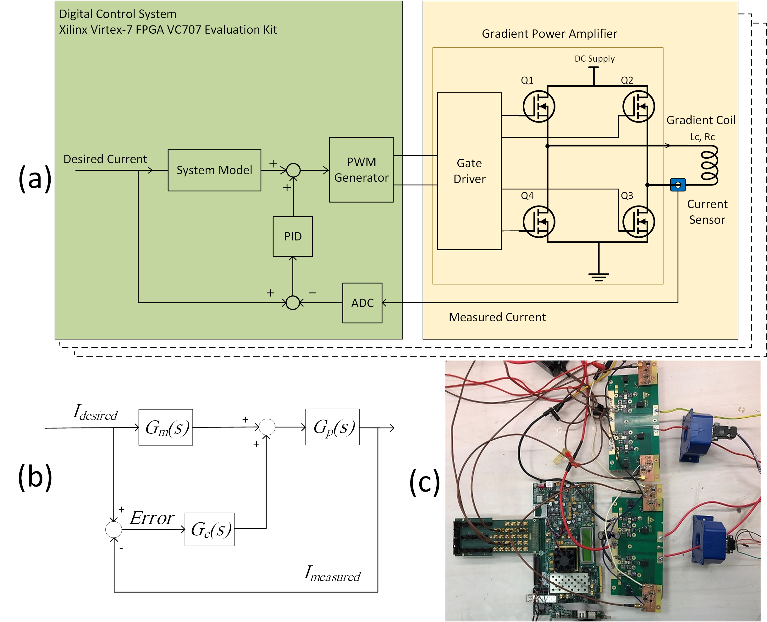
The block diagram of gradient array system is shown in Fig.1. A typical trapezoid current waveform is used to drive two channels of z-gradient array coils. The hardware limitations are considered in designing input current waveforms. The first-order model including mutual coupling provides the required voltage. This model acts like a multi-input-multi-output (MIMO) proportional-derivate (PD) controller in the open-loop configuration. The parameters were determined by measuring self-inductance, mutual inductance, and resistance of coils.
$$\left[{\begin{array}{*{20}{c}}{{v_1}\left(t\right)}\\{{v_2}\left(t\right)}\end{array}}\right]=\left[{\begin{array}{*{20}{c}}{{L_1}}&M\\M&{{L_2}}\end{array}}\right]\left[{\begin{array}{*{20}{c}}{\frac{{d{i_1}\left(t\right)}}{{dt}}}\\{\frac{{d{i_2}\left(t\right)}}{{dt}}}\end{array}}\right]+\left[{\begin{array}{*{20}{c}}{{R_1}}&0\\0&{{R_2}}\end{array}}\right]\left[{\begin{array}{*{20}{c}}{{i_1}\left(t\right)}\\{{i_2}\left(t\right)}\end{array}} \right]$$
The close-loop feedback PID controller is used in parallel with the feedforward model which will update the required voltage to minimize the error between desired input and measured output. The transfer function analysis can be used for the determination of PID parameters.
$${I_m}\left(s\right)={\left[{{\rm{I}}+{G_c}\left(s\right){G_p}\left(s\right)}\right]^{-1}}\left[{{G_m}\left(s\right){G_p}\left(s\right)+{G_c}\left(s\right){G_p}\left(s\right)}\right]{I_d}\left(s\right)$$
Where, G_m(s), G_p(s), G_c(s) are transfer functions for the model, gradient coil with amplifier and PID controller respectively. Assuming no mutual coupling and single-input-single-output PID, the transfer function for channel 1 is as follow:
$$\frac{{{I_{m1}}\left(s\right)}}{{{I_{d1}}\left(s\right)}}=\frac{{{G_{m1}}\left(s\right){G_{p1}}\left(s\right)+{G_{c1}}\left(s\right){G_{p1}}\left(s\right)}}{{1+{G_{c1}}\left(s\right){G_{p1}}\left(s\right)}}$$
G_m1(s) is the model of channel 1 which is the inverse of G_p1(s) in the ideal case. Assuming G_m1(s)G_p1(s) ≈ 1, to have an accurate regulation on the output current, |G_c1(s)G_p1(s)| >> 1. Therefore, by increasing the gain of controller (G_c1) at the operating frequency, the measured current approaches to the desired one. The PID block changes the desired voltage in a real-time fashion which results in a change in the duty cycle of PWM signals. The transfer function analysis reveals two things, (a) if the model can be determined exactly, there is no need for the feedback loop. However, in the real case, the imperfections and measurement errors affect the system which cannot be modeled, (b) considering mutual coupling in the model is not compulsory and the feedback loop can compensate for it.
The whole control system was designed digitally using the Xilinx VC707 FPGA board. The PWM signals were generated with 15-bit resolution and duty cycles can be controlled in the range of picosecond. A home-built full-bridge power amplifier with 1 MHz effective switching frequency is used to provide 10V and 8A at the output.

Results

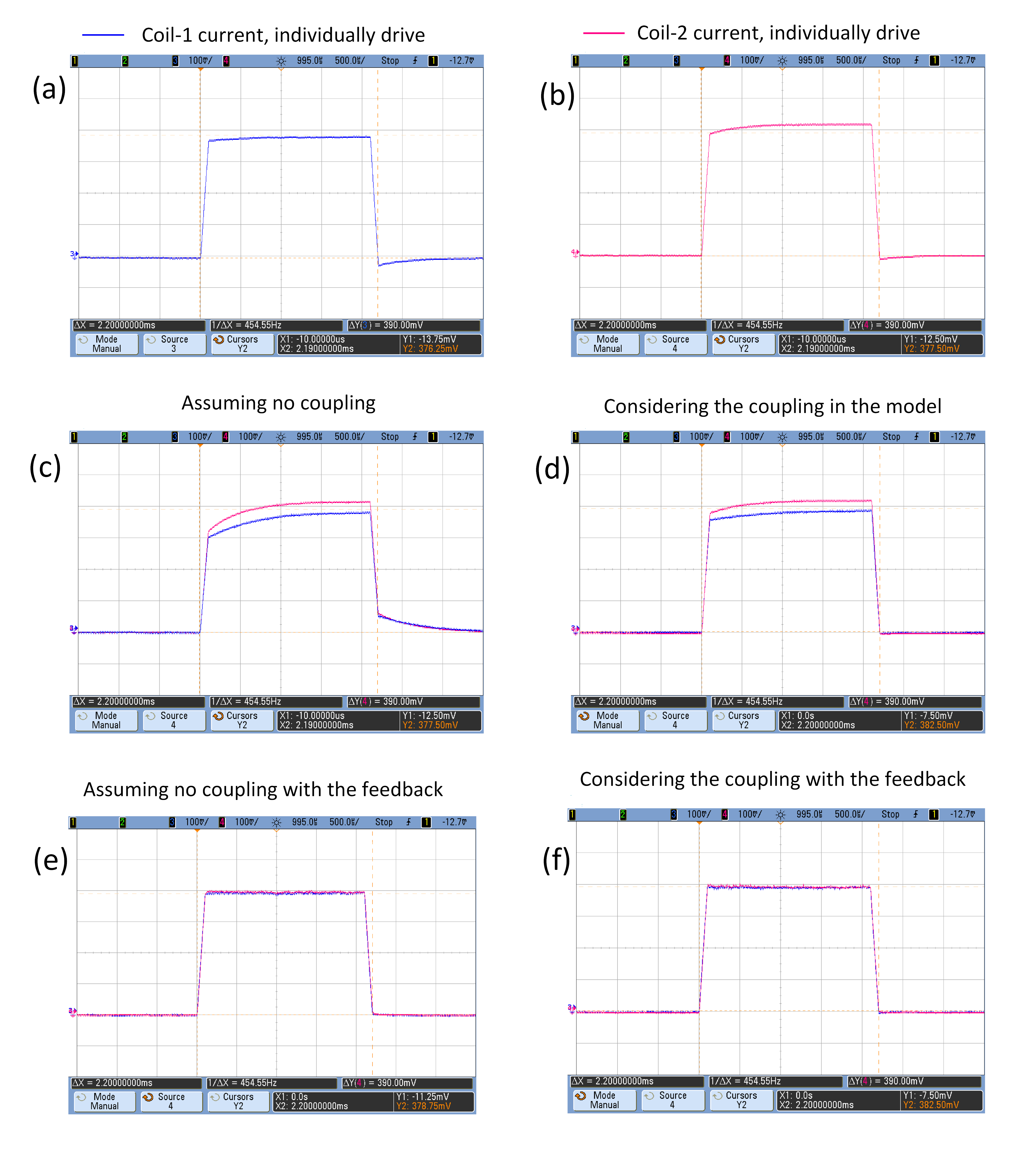
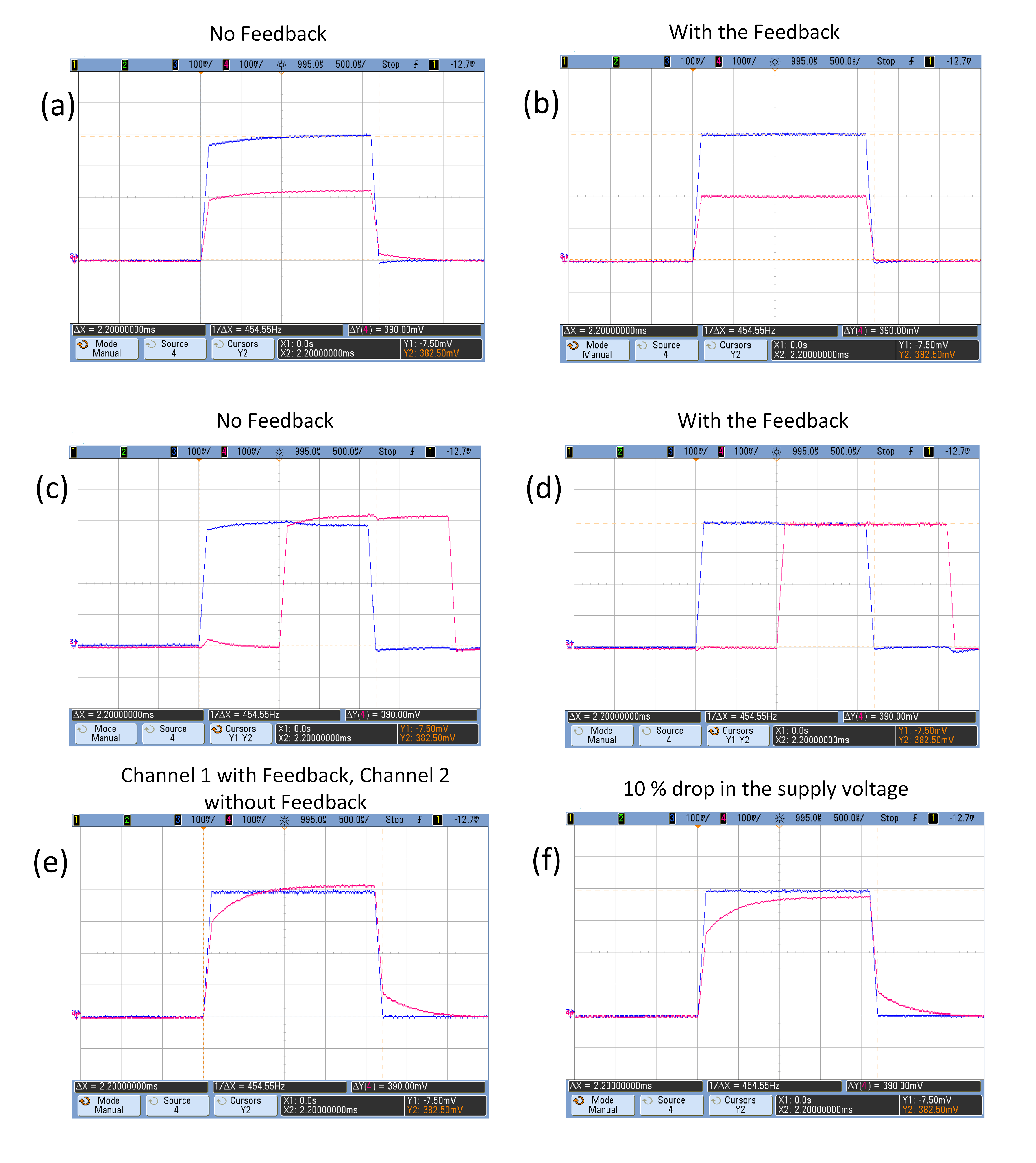
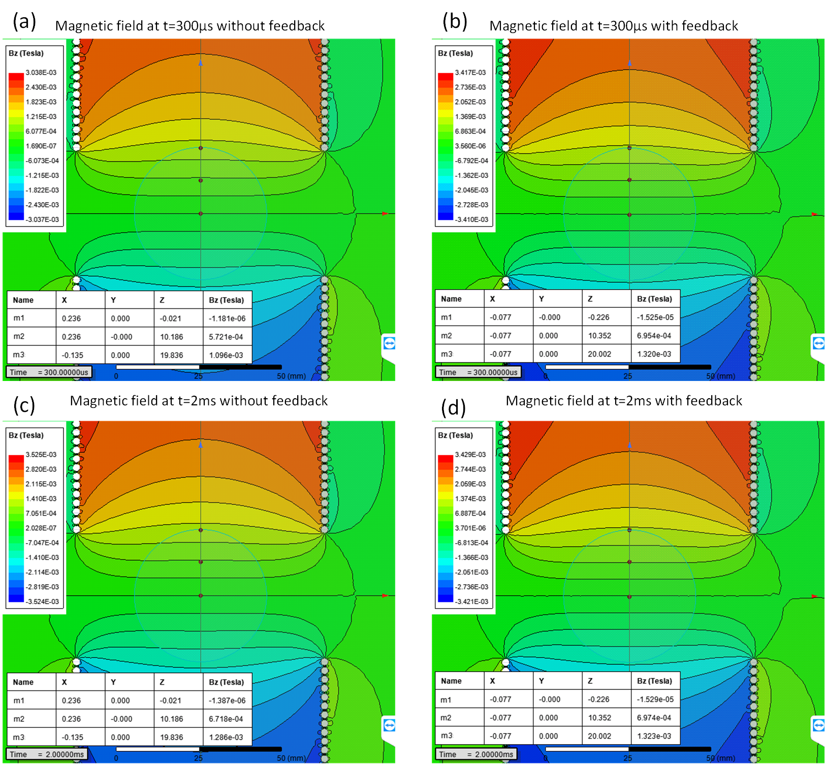
The coil currents were measured by fluxgate current sensors (IT 205-S) and results are shown on the oscilloscope. The output currents are shown for driving the coils individually (no mutual coupling, no feedback, Fig. 2a,b) and simultaneously (Fig. 2c,d). Due to measurement errors in the model parameters and not considering GPA, the desired waveform cannot be achieved. It is possible to change the parameters manually and iteratively to get the desired one, however, the model may change caused by time-varying parameters such as temperature. The output currents in the presence of feedback loop are depicted in Fig. 2e,f. The feedback performance is tested in two cases, input currents are applied with (a) different amplitudes, same phases (Fig. 3a,b), (b) same amplitudes, different phases (Fig. 3c,d). The robustness of system is tested for droop in the supply voltage (Fig. 3e,f). The simulation of magnetic field profiles generated by actual current values on the coils, with and without the controller is shown in Fig.4.

Discussion and Conclusion

In this work, to compensate the mutual coupling and undesired imperfections, a real-time digital PID controller design is proposed. The feedback loop in combination with feedforward PD model provides the desired voltage which has to be applied to the coils. The PID controller can adjust the PWMs duty cycle in order to minimize the error between desired and measured current. Although adding PID can make the correction for undesired distortions, the stability of the system has to be considered in the presence of the controller. To have a perfect current regulation, the gain of controller has to be high which may cause instability in the system or exceeds the GPAs limitation.

Acknowledgements

No acknowledgement found.