Introduction

Electromagnetic noise in ultra-low field (ULF) MR is orders of magnitude larger than in high field MRI, necessitating the development of ULF-MR methods for noise reduction¹. The traditional approach has been to isolate the instrument from the external environment using a magnetically shielded enclosure², which is expensive and hinders portability. To overcome these drawbacks, a software-gradiometer setup with a convolutional neural network (CNN) framework is proposed for noise reduction. Here, the approach is introduced and the results from an ULF-MR experiment presented.

Methods-theory

Our goal is to remove background electromagnetic noise from the NMR acquisition using measurements made by three background coils. The variables involved in the detection can be seen by looking at the equations governing the signal induced in a coil placed near the sample (S₀), and in the three background coils (S₁, S₂, S₃) such that
$$ S_{i}=-\frac{\partial }{\partial t}\int_{V_{1}}^{} B_{i}\cdot J_{s}dV +\sqrt{4kT_{c}\triangle f R_{i}} - \frac{\partial }{\partial t}\int_{V_{2}}^{} B_{i}\cdot M_{s}dV,i=0,1,2,3 $$
The NMR signal is determined by the sensitivity of the NMR coil (B₀) and the sample magnetization (M_s). J_s is the noise source, B₁, B₂ and B₃ are magnetic field sensitivities associated with each of the three background coils, T_c is the temperature, k is the Boltzmann constant, Δf is signal bandwidth, R_i is the resistance of each coil i, V₁ is the space of the noise sources and V₂ is the volume of the sample. There are two types of noise sources in Eq.1: The background noise from J_s and the thermal noise caused by resistance R_i.
Thermal noise is much smaller than ambient noise so the second term of Eq.1 can be ignored. The third term can also be neglected as the background coils are far from the sample. Hence, the estimated noise signal can be simplified to a weighted contribution of the first term such that:
$$S_{syn}=\sum_i^3-\frac{\partial }{\partial t}\int_{V_{1}}^{}\alpha_{i}B_{i}\cdot J_{s}dV (2)$$
which can then be solved by the optimization problem
$$min_{\alpha_{1}\alpha_{1}\alpha_{1}}(\int_{V_{1}}^{}B_{0}\cdot J_{s}dV- S_{syn})(3)$$
Here α_i are coefficient vectors of that relate the noise on the NMR coil with the noise recorded by each ambient coil. Eq.3 is the cost function for finding optimal values for αi.
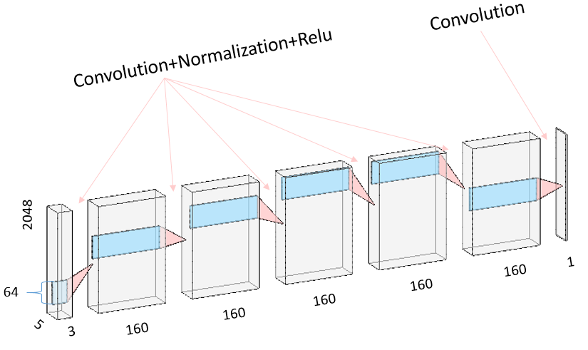
Solving for αi in Eq.2&3 is complicated because of the temporal, spatial and frequency dependence of the noise and the limitations of the acquisition accuracy. Hence, we opted to use a CNN as it can implement a large variety and number of filters and convolution operations that can cater for acquisition differences between coils.

Methods-Experiment

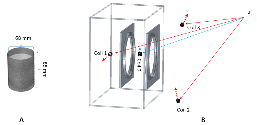
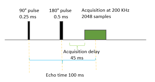
Three air-core magnetometers³ were built for background field measurements in addition to a magnetometer placed at the sample (Fig1).
A resistive Helmholtz pair of coils was used to generate a static magnetic field of 0.186 mT (Fig.1B). The setup, including the four magnetometers, was partially shielded using transformer steel sheets to reduce off-resonance effects arising from the strong static magnetic fields produced by other equipment in the vicinity of the laboratory. All coils were identical. The signal S₀ was acquired using a Magritek Aurora console. Synchronously, background coil measurements were made using a NI-DAC (USB-6259). The spin echo pulse sequence (Fig.2) was used for the experiment. All acquisitions recorded 2048 samples per coil at 200 samples/s. 1000 spin echoes were generated without an NMR sample and 64 echoes were generated with a 25 ml water phantom in-situ. Measurements without the sample were divided into 900, 64 and 32 instances, and respectively used for training, testing and validating the CNN. The CNN structure details can be seen in Fig.3. The CNN loss function was calculated as the mean squared error between predicted and acquired noise without the sample. 200 training epochs were performed with each employing all 900 datasets. The 64 datasets acquired with the water phantom in-situ were fed into the trained CNN. Predicted noise signals were individually subtracted from their corresponding water NMR signals. These 64 denoised NMR signals were averaged and compared with the averaged original counterpart.

Results

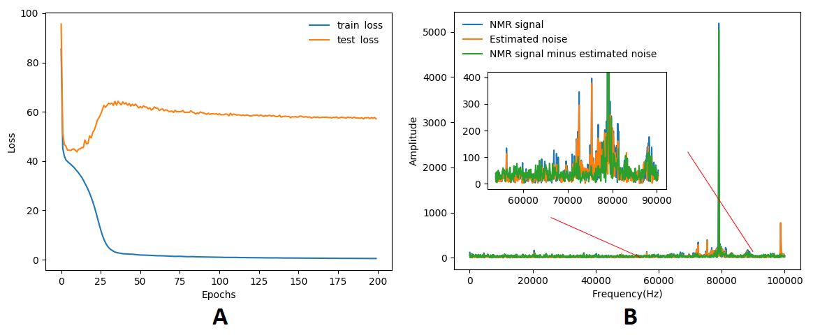
The CNN training result is shown in Fig.4A. The training and testing losses indicate the prediction accuracy for known and unknown datasets respectively. NMR Spectra with and without noise attenuation and estimated noise are shown in Fig.4B. At the NMR signal frequency the mean and standard deviation of the amplitude of 64 signals was 5264 and 743 before subtracting the estimated noise, and 5109 and 414 after noise subtraction.

Discussion

The training loss of the CNN converges quickly (Fig.4A), however the testing loss has a small oscillation and converges slowly after 30 epochs. These noise peaks distributed in frequencies neighbouring the NMR signal (Fig.4B) are significantly reduced after the noise attenuation. Attenuation is largest in the 80 kHz neighbourhood of the NMR signal. No significant improvement can be noticed in the NMR signal because ambient noise was very low at that frequency in performed experiments. Collection of larger datasets to improve the training results and the use of more sensitive sensor coils with lower thermal noise are expected to improve the performance of the software-gradiometer.

Conclusion

Presented initial results suggest that CNNs can be used with software-gradiometry to reduce electromagnetic ambient noise. This approach has the potential to reduce size, weight and cost of ULF-MR instruments.

Acknowledgements

No acknowledgement found.