4194
A conditional safety margin to reduce the peak local SAR overestimation due to the conventional safety factor
E. F. Meliado1,2,3, A. Sbrizzi1,2, C.A.T. van den Berg2,4, B. R. Steensma1,2, P.R. Luijten1, and A. J. E. Raaijmakers1,2,5
1Department of Radiology, University Medical Center Utrecht, Utrecht, Netherlands, 2Computational Imaging Group for MR diagnostics & therapy, Center for Image Sciences, University Medical Center Utrecht, Utrecht, Netherlands, 3Tesla Dynamic Coils BV, Zaltbommel, Netherlands, 4Department of Radiotherapy, Division of Imaging & Oncology, University Medical Center Utrecht, Utrecht, Netherlands, 5Biomedical Image Analysis, Dept. Biomedical Engineering, Eindhoven University of Technology, Eindhoven, Netherlands
1Department of Radiology, University Medical Center Utrecht, Utrecht, Netherlands, 2Computational Imaging Group for MR diagnostics & therapy, Center for Image Sciences, University Medical Center Utrecht, Utrecht, Netherlands, 3Tesla Dynamic Coils BV, Zaltbommel, Netherlands, 4Department of Radiotherapy, Division of Imaging & Oncology, University Medical Center Utrecht, Utrecht, Netherlands, 5Biomedical Image Analysis, Dept. Biomedical Engineering, Eindhoven University of Technology, Eindhoven, Netherlands
Synopsis
The introduction of a linear safety factor to address peak local SAR uncertainties (e.g. inter-subject variation and modeling inaccuracies) bears one considerable drawback: it often results in over-conservative scanning constraints. In this work, we present a more efficient and probabilistic approach to define a variable safety margin based on the conditional probability density function of the true peak local SAR value given the estimated peak local SAR value. Results show that the proposed approach leads to a reduction of peak local SAR overestimation up to 30%.
PURPOSE
The assessment of 10g-averaged peak local SAR (pSAR) for MR imaging with multi-transmit arrays is typically done by off-line numerical simulations using one or several generic models1. Subsequently, the post-processed simulation results can be used for on-line pSAR estimation2,3. To compensate for the discrepancies between the generic simulation models and the subject under examination an additional safety factor is required to avoid pSAR underestimation. This approach is suboptimal as illustrated by Figure 1. Here, for 23 simulation models4 with each 250 random phase settings, the true pSAR (pSART) is plotted versus the estimated pSAR (pSARE, based on the generic model Duke5). pSARE is often lower than pSART so a safety factor is applied which transforms pSARE into a corrected pSARE value (pSARE,C) as indicated by the red line in Figure 1. pSAR underestimation is now avoided as the scatter points are below the red line. However, this representation clearly shows that for large pSARE values, the pSARE,C heavily overestimates the pSART. In this study we present the conditional safety margin as an alternative approach for the linear safety factor based on probability theory.THEORY
The scatter plot in Figure 1 represents samples from the joint probability distribution of pSARE and pSART, which is described by the probability density function $$$f_{E,T}(pSAR^E,pSAR^T)$$$. When we estimate a pSARE value, we would like to know the probability of pSAR underestimation i.e. $$$P(pSAR^T>pSAR^E)$$$. Thus, we need to know the conditional probability density function $$$f_{T|E}(pSAR^T|pSAR^E)$$$ which is the probability distribution of pSART for a given pSARE. This function is calculated in Eq. [1] where $$$f_E(pSAR^E)$$$ is the (marginal) probability density function of pSARE (regardless of pSART). See Figure 2.$$f_{T|E}(pSAR^T|pSAR^E)=\frac{f_{E,T}(pSAR^E,pSAR^T)}{f_E(pSAR^E)}$$ [1]
Now the probability $$$P_{underest}$$$ that pSART is actually larger than some estimated value pSARE=E1 is given by [2].
$$P_{underest}=P(pSAR^T>E_1|pSAR^E=E_1)=\int_{E_1}^{\infty} f_{T|E}(pSAR^T|pSAR^E=E_1)dpSAR^T$$ [2]
METHODS
The probability density functions can be estimated from the observed data. Therefore, a representative set of (pSART,pSARE) samples is generated by means of our database of 23 subject-specific models4 with an 8-fractionated dipole array6,7 for prostate imaging at 7T.For each of the 23 models, driving the array with uniform input power (8×1W) and random phase settings, 250 pSART values are determined. Three state-of-the-art methods are used to estimate the pSARE values: 1) using just the generic model “Duke”5; 2) using our model library to assess the maximum pSAR value over all models; 3) using a recently published deep learning-based method, where the SAR distribution is determined by a deep learning network with an acquired B1+-map as an input8
Conditional Safety Margin
The pairs (pSARE,pSART) are samples from the joint probability density function $$$f_{E,T}(pSAR^E,pSAR^T)$$$, which can be modelled as a Gaussian mixture (Figures 2.a,b). All pSARE values are samples from the marginal probability density function $$$f_E(pSAR^E)$$$ and follow what seems to be a Gamma distribution (Figure 2.c). Therefore, using equation [2], the conditional probability density function can be calculated for each possible estimated pSARE=E1 value and used to numerically determine a corrected pSARE,C value with a probability of underestimation equal to an arbitrary (small) ε (Figure 2.d).
$$$Find$$$ $$$pSAR^{E,C}$$$ $$$such$$$ $$$that$$$
$$P(pSAR^T>pSAR^{E,C}|pSAR^E=E_1)=\int_{pSAR^{E,C}}^{\infty} f_{T|E}(pSAR^T|pSAR^E=E_1)dpSAR^T=\epsilon$$ [3]
This corrected pSARE,C value represents our conditional safety margin (CSM).
Performance Evaluation
To assess the performance of the conditional safety margin, a larger test set (23×1000=23000 test samples) is generated and the mean overestimation of the conditional safety margin is evaluated and compared to the mean overestimation of the corrected pSAR values using the linear safety factor (LSF)8.
RESULTS AND DISCUSSIONS
To determine the joint and marginal probability density functions, for each considered pSAR estimation method, the scatter plot pSART versus pSARE is fitted with a mixture of five Gaussian distributions, and the pSARE histogram is fitted with a Gamma distribution. Subsequently, the conditional safety margin is evaluated for ε=0.001.Figure 3.a shows the scatter plot pSART versus pSARE using the generic model, and the corrected pSARE,C values. The red line is the corrected pSARE,C by LSF and the green line is the corrected pSARE,C by CSM. Similar scatter plots for the model library and the deep learning method are shown in Figures 3.b and 3.c respectively.
Figure 3 clearly shows that the suggested approach is reducing overestimation because the green line remains closer to the distribution of actually expected pSART values. The mean overestimation over all models and drive settings for each method is reported in Figure 3.d.
Results show that the conditional safety margin allows to reduce the mean overestimation from 108% to 89% using the generic model (18% reduction), from 104% to 83% using the model library (20% reduction) and from 57% to 41% with the deep learning method (28% reduction). Note that these are averaged values. For individual cases with high pSARE values, the reduction in overestimation may reach up to 40%.
CONCLUSIONS
An alternative, probabilistic approach for peak local SAR correction is proposed. It allows to define a variable safety margin to deal better with peak local SAR uncertainties. It reduces the average overestimation up to 30% compared to the more conventional safety factor.Acknowledgements
No acknowledgement found.References
- Homann H, Börnert P, Eggers H, Nehrke K, Dössel O, Graesslin I. Toward individualized SAR models and in vivo validation. Magn Reson Med. 2011;66(6):1767-1776.
- Graesslin I, Homann H, Biederer S, et al. A specific absorption rate prediction concept for parallel transmission MR. Magn Reson Med. 2012;68(5):1664-1674.
- Eichfelder G, Gebhardt M. Local specific absorption rate control for parallel transmission by virtual observation points. Magn Reson Med. 2011;66(5):1468-1476.
- Meliadò EF, van den Berg CAT, Luijten PR, Raaijmakers AJE. Intersubject specific absorption rate variability analysis through construction of 23 realistic body models for prostate imaging at 7T. Magn Reson Med. 2019;81(3):2106-2119.
- Christ A, Kainz W, Hahn EG, et al. The Virtual Family—development of surface‐based anatomical models of two adults and two children for dosimetric simulations. Phys Med Biol. 2010;55:N23–N38.
- Steensma BR, Luttje M, Voogt IJ, et al. Comparing Signal-to-Noise Ratio for Prostate Imaging at 7T and 3T. J Magn Reson Imaging. 2019;49(5):1446-1455.
- Raaijmakers AJE, Italiaander M, Voogt IJ, Luijten PR, Hoogduin JM, et al. The fractionated dipole antenna: A new antenna for body imaging at 7 Tesla. Magn Reson Med. 2016;75:1366–1374.
- Meliadò EF, Raaijmakers AJE, Sbrizzi A, et al. A deep learning method for image‐based subject‐specific local SAR assessment. Magn Reson Med. 2019;00:1–17.
Figures
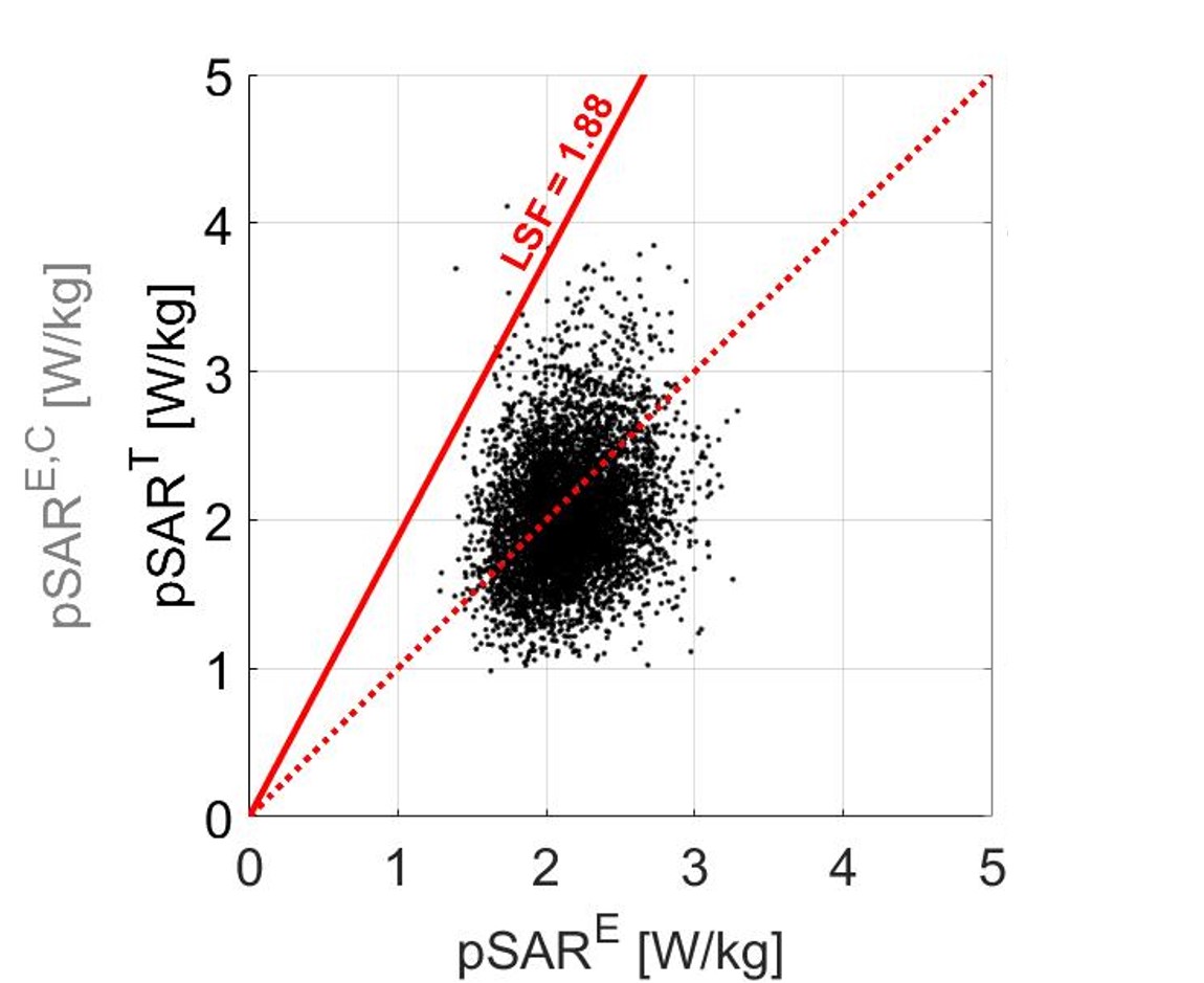
Figure 1: Scatter plot of the true
pSART versus the estimated pSARE using the generic model
Duke with random phase settings. The red line is the
corrected pSARE,C by the linear safety factor. The red dotted line indicates where estimated pSARE levels and true pSART levels are equal. Points above the line represent true
pSART levels larger than estimated (underestimation
error). The linear scaling factor (LSF) is chosen such that 99.9% of the points
are below the red solid line and underestimation is avoided. For large pSARE values, this
results in very large pSARE,C values.
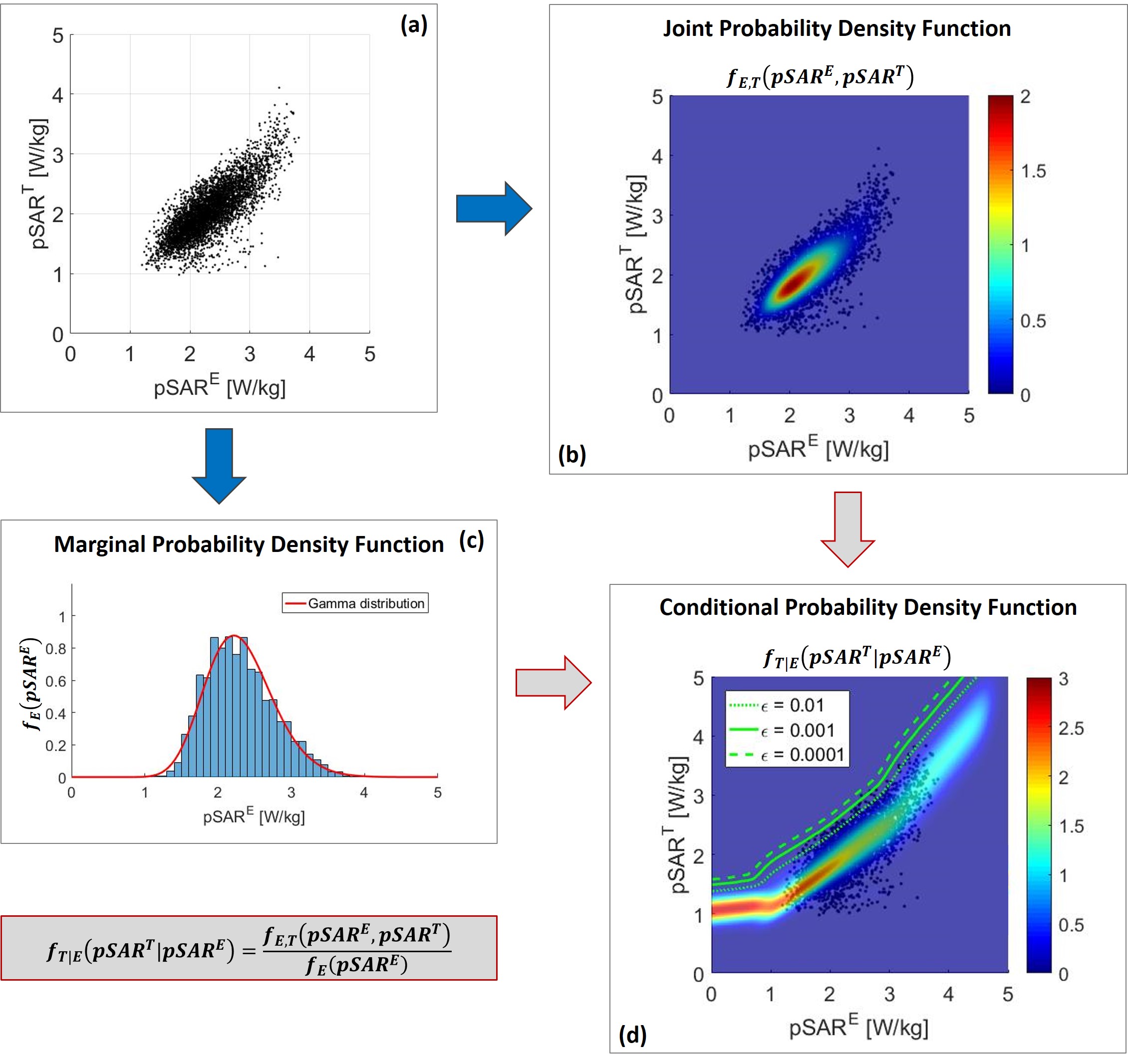
Figure
2: (a)
Scatter plot of the true
pSART versus the estimated pSARE using the deep learning
method. (b) Joint probability density function fE,T(pSARE, pSART) of the estimated and true pSAR values.
(c) Marginal probability density function fE(pSARE) of the estimated pSAR values. (d) 2D conditional probability density function fT|E(pSART|pSARE) obtained combining the 1D conditional probability density
functions for each possible pSARE value.
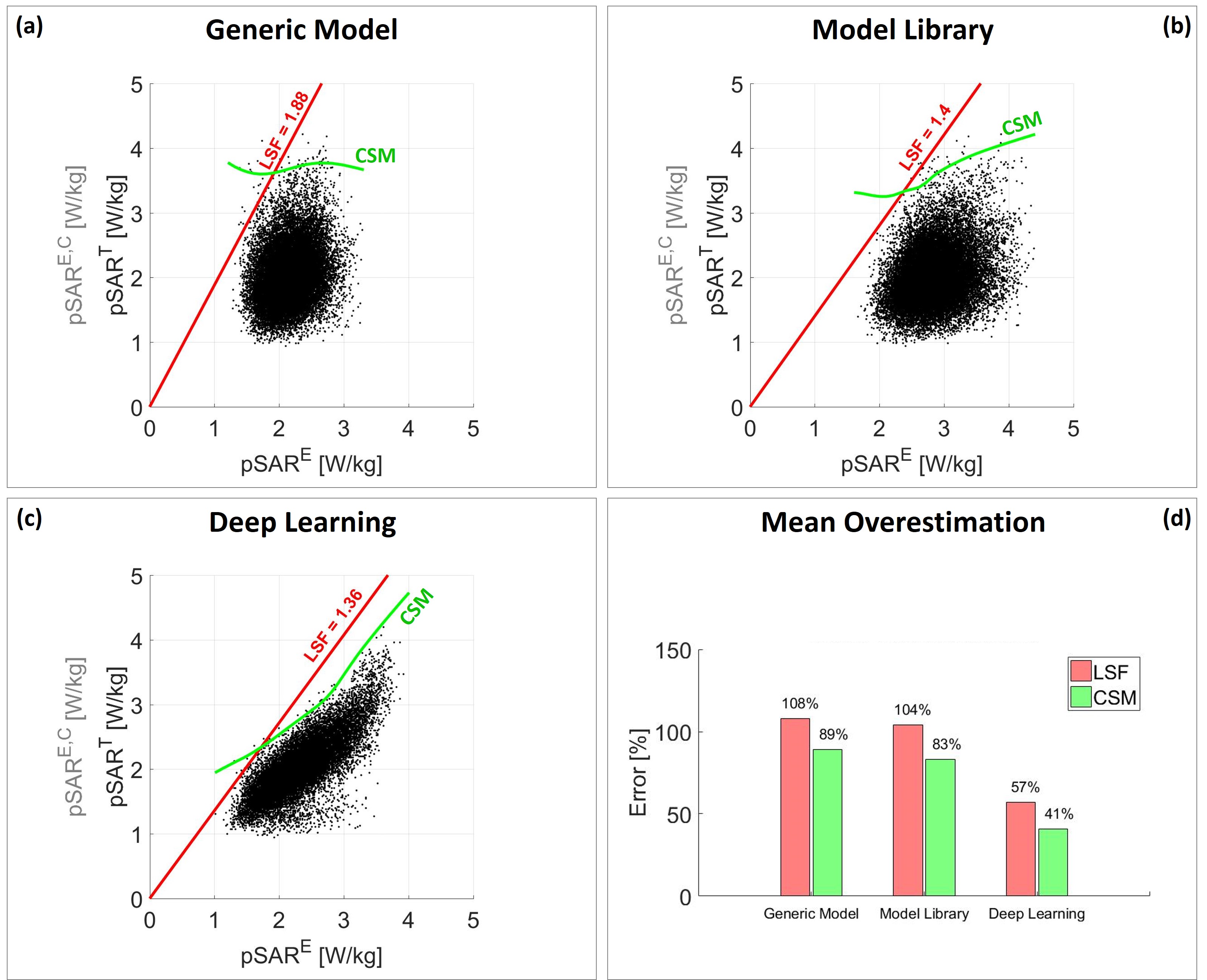
Figure 3: Scatter plots of the true
pSART versus the estimated pSARE and the corrected pSARE,C
values using: (a) generic body model
Duke; (b) the model library to assess the maximum pSAR value over all models; (c)
the deep learning-based method. The red line represents the corrected pSARE,C
by the linear safety factor LSF. The green line is the corrected pSARE,C
by the conditional safety margin CSM. (d) Bar plot of the mean overestimation error
for each pSAR estimation method.