4191
Intra- and inter- brain RF heating prediction with the Non-Invasive Temperature Estimation (NITE) method
Julie M. Kabil1, Sairam Geethanath1, and J. Thomas Vaughan1
1Columbia Magnetic Resonance Research Center, Columbia University, New York, NY, United States
1Columbia Magnetic Resonance Research Center, Columbia University, New York, NY, United States
Synopsis
Radiofrequency-induced heating is a major concern in MRI and these risks widely vary between patients. Therefore, we propose a personalized, deep learning temperature estimation method. After electromagnetic and thermal simulation on two human models in a radiofrequency coil, we trained a neural network on one brain slice to predict internal brain temperatures, using the following features: tissue properties, distance to four surface sensors and the corresponding four surface temperatures. Fast testing performed on both intra- and inter- brain slices revealed similar thermal maps compared to simulated maps. Ongoing work targets a better generalization to different anatomies and in vivo experiments.
Introduction
Safe and time-efficient MRI scans remain challenging as radiofrequency heating notably depends on patients’ anatomy1-3. We propose a non-invasive and precision approach to temperature, supported by deep learning4,5 and tested on two different brains. Our goal is to accurately predict internal body temperature based on patient-specific parameters such as tissue distribution and surface temperature. The principle behind our Non-Invasive Temperature Estimation (NITE) method is as follows: consider a brain slice inside which the temperature distribution is unknown (N points). Let us now consider Ns surface temperature sensors. Each internal point Np is linked to each surface sensor by an imaginary line divided in q segments, to take into account the tissue distribution and parameters - permittivity, conductivity, density ($$$\epsilon$$$, $$$\sigma$$$, $$$\rho$$$) - along this line. The temperature profile for the Np point can be written as: $$$P_N{{_p-}}{_N}_{{_S}{_1}} = [\epsilon(\overrightarrow{r}),\sigma(\overrightarrow{r}),\rho(\overrightarrow{r}),\parallel N{{_p-}}N_{{_S}{_1}} \parallel_2, N_{{_S}{_1}}(\overrightarrow{r},T{_{N}}_{{_S}{_1}})]$$$. Finally, we can describe the mapping of internal temperature as an inverse problem. We consider a neural network classification problem with a defined precision of 0.1°C, train a neural network on one brain slice using the features mentioned above, and then test this model on other slices to predict the unknown internal temperatures.Methods
Using the CST Studio Suite software (Dassault Systèmes, France), a 4T TEM head coil was modeled and two different numerical human models (Visible Human Male HUGO and Visible Human Female NELLY) were imported in this coil with a 0.8 mm resolution. An electromagnetic and thermal co-simulation was performed and temperature maps were obtained for both brains, on 9 axial slices (5 HUGO’s, 4 NELLY’s). The slices were manually segmented in CST with different tissue types (White Matter, Gray Matter, CerebroSpinal Fluid, Bone, Muscle, Fat, Skin, Blood, Air) as seen in Figure 1a (HUGO) and Figure 1b (NELLY). They were then imported in Matlab to map the tissue properties to each slice: permittivity, conductivity, density. The thermal maps obtained from CST were imported in Matlab for data preparation for the deep learning training (Figure 2). An array of 35 features for each point was the input: 33 tissue properties (11 segments having 3 properties each), 1 norm distance to each of the four surface sensors, 1 surface temperature value. The output was the internal temperature for each point. The neural network was implemented in TensorFlow with 3 layers, a total of 270 nodes, a ReLU (Rectified Linear Unit) activation function, a learning rate of 0.0001 and 800 epochs (Figure 3a). Random dropout was implemented to prevent overfitting and improve the generalization to unseen slices. The training was done on one slice from the HUGO model: after the training was completed, testing was performed on the other slices from both HUGO and NELLY. The generated temperature maps were then compared with the temperature maps obtained from CST (Figure 3b). Additionally, the time necessary to run the full CST simulation and NITE was examined.Results
The cost at the final epoch was 0.18, the training and testing accuracy were 93% and validation loss was 0.19. The solution converged as the validation loss reached a minimum. Simulated and predicted temperature maps are visible in Figure 4a (HUGO) and Figure 4b (NELLY). Figure 5 shows the quantitative comparison between the same simulated and predicted temperature maps both for HUGO (Figure 5a) and NELLY (Figure 5b). The left picture shows the correlation between CST and NITE. The right picture shows the temperature difference between CST and NITE: positive and negative values respectively show where NITE is overestimating and underestimating temperature compared to CST. The CST full simulation was in the order of magnitude of hours, whereas once the training was done (in less than an hour) the thermal map prediction was done in milliseconds.Discussion
The closer (anatomically) a test slice is from the training slice, the more accurate the prediction is. Intra-brain results obtained with the first HUGO test slice (Figure 4a – upper row) show comparable results between CST and NITE, which is consistent with the similarities existing between the training and test slice. In NELLY’s test slices, some tissue types who were present in the training slice are not present in NELLY’s slices (Blood and Air): this has an influence on inter-brain testing performance and the ability to generalize. However, hotspots predictions are encouraging especially when considering Figure 5: NITE tends to overestimate rather than underestimating temperature, while still accurately locating major hotspots. Finally, the time comparison is in favor of NITE which generates temperature maps in milliseconds compared to the hours needed for CST. One challenge to overcome is to use several brain slices to train the network. Nevertheless, deep learning has shown promising capabilities in other safety estimation methods (SAR-wise)6, and our current work also supports the use of artificial intelligence to tackle RF safety problems. Finally, this work is an in silico study, however we plan to test our method in vivo using MRI images acquisition.Conclusion
This study demonstrates the potential of this deep learning-based temperature estimation method to generalize to different brains, while keeping the computational cost low compared to traditional numerical simulations: in vivo experiments will allow to definitely conclude on the potential of the method.Acknowledgements
No acknowledgement found.References
1. Rieke V et al. MR thermometry. J Magn Reson Imaging. 2008;27(2):376-90. 2. Shrivastava D et al. Stepping Towards Subject Specific Temperature Modeling to Improve Thermal Safety in Clinical and Ultra-High Field MRI. Proceedings of the ASME 2013 Conference on Frontiers in Medical Devices: Applications of Computer Modeling and Simulation, 2013. 3. Shrivastava D et al. In vivo radiofrequency heating in swine in a 3T (123.2-MHz) birdcage whole body coil. Magn Reson Med. 2014;72(4):1141–1150. 4. Geethanath S, Kabil J, Vaughan JT. Abstract, ISMRM Workshop on Machine Learning 2018. 5. Kabil J, Geethanath S, Vaughan JT. Abstract, ISMRM 2019. 6. Meliadò EF et al. A deep learning method for image‐based subject‐specific local SAR assessment. Magn Reson Med. 2019; 00: 1– 17.Figures
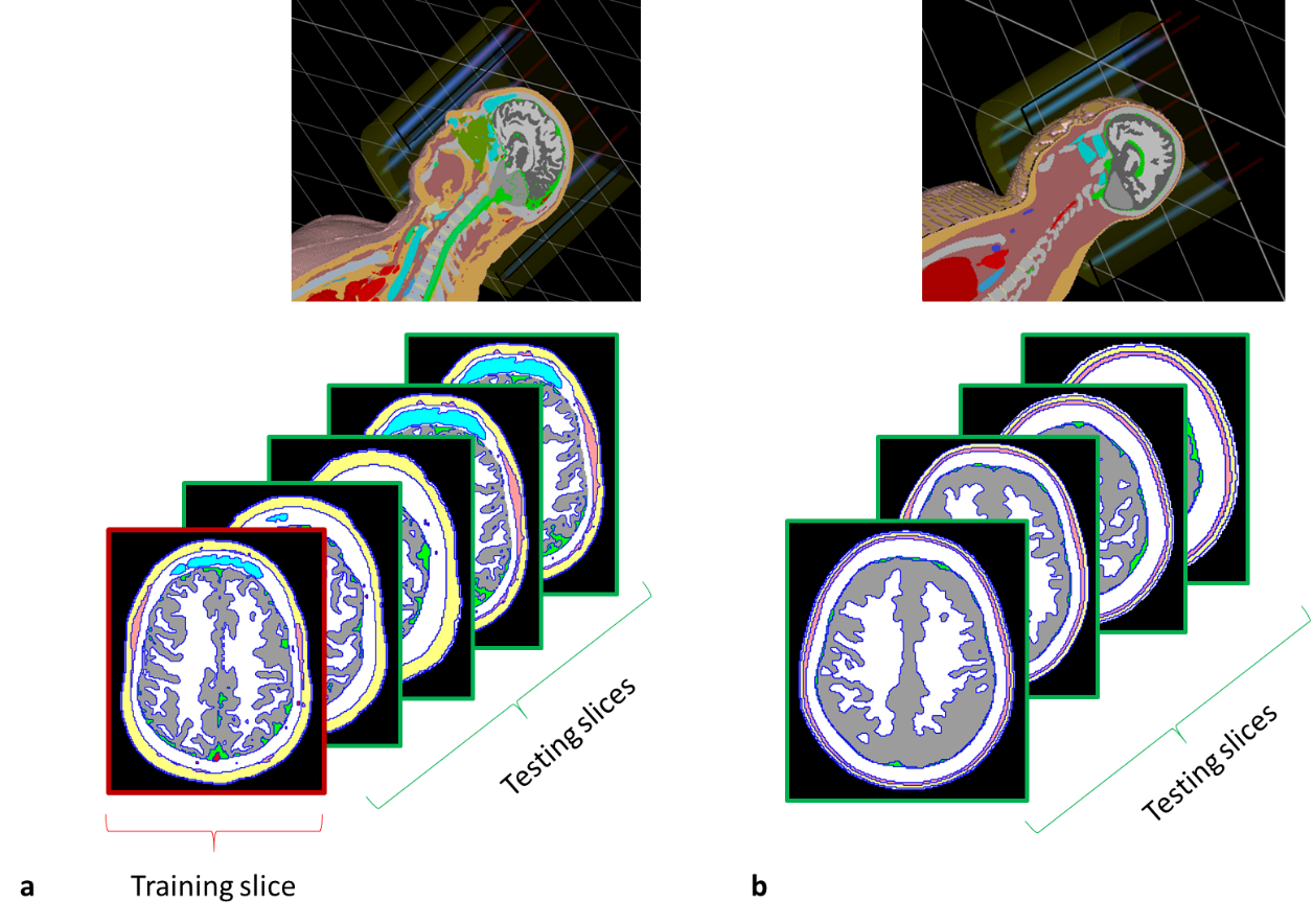
Figure 1: Data acquisition in CST. a. HUGO model inside the TEM head coil, segmented training slice
(red), segmented intra-brain testing slices (green). b. NELLY model inside the TEM head coil, segmented inter-brain
testing slices (green).
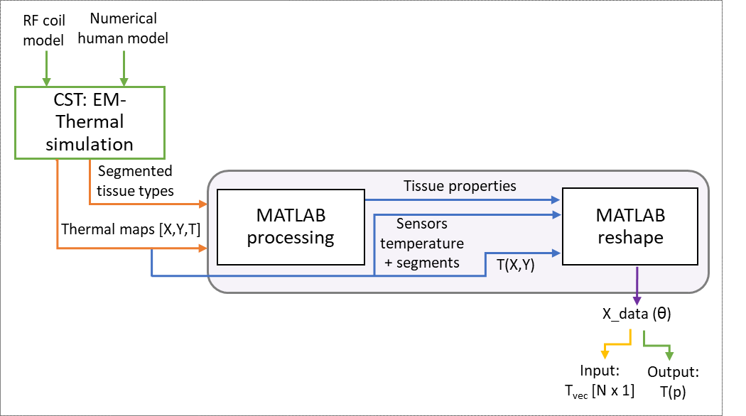
Figure 2: Data preparation for
deep learning. After reshaping, all the data from CST is put in a matrix
including the input (features) and output (internal temperatures) for the
training phase; and only the input for the testing phase.
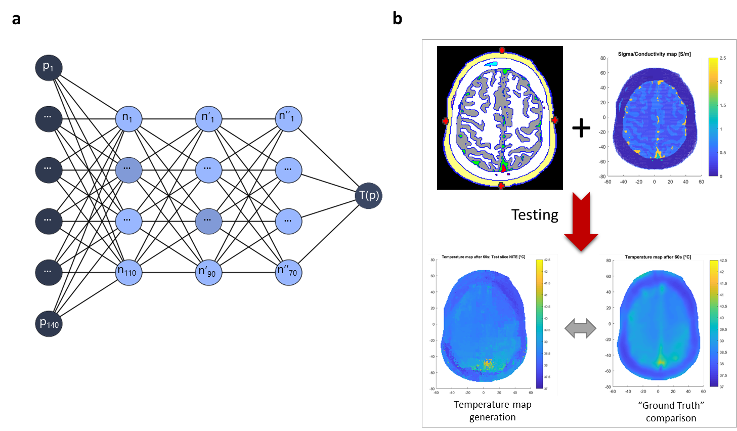
Figure 3: Training and testing process.
a. Deep neural network architecture
for training. b. Testing phase: the
tissue distribution along with the surface temperature sensors (red points) are
fed to the model, which reconstructs a predicted temperature map which is in turn
compared to the “Ground Truth” map (here, the simulated map).
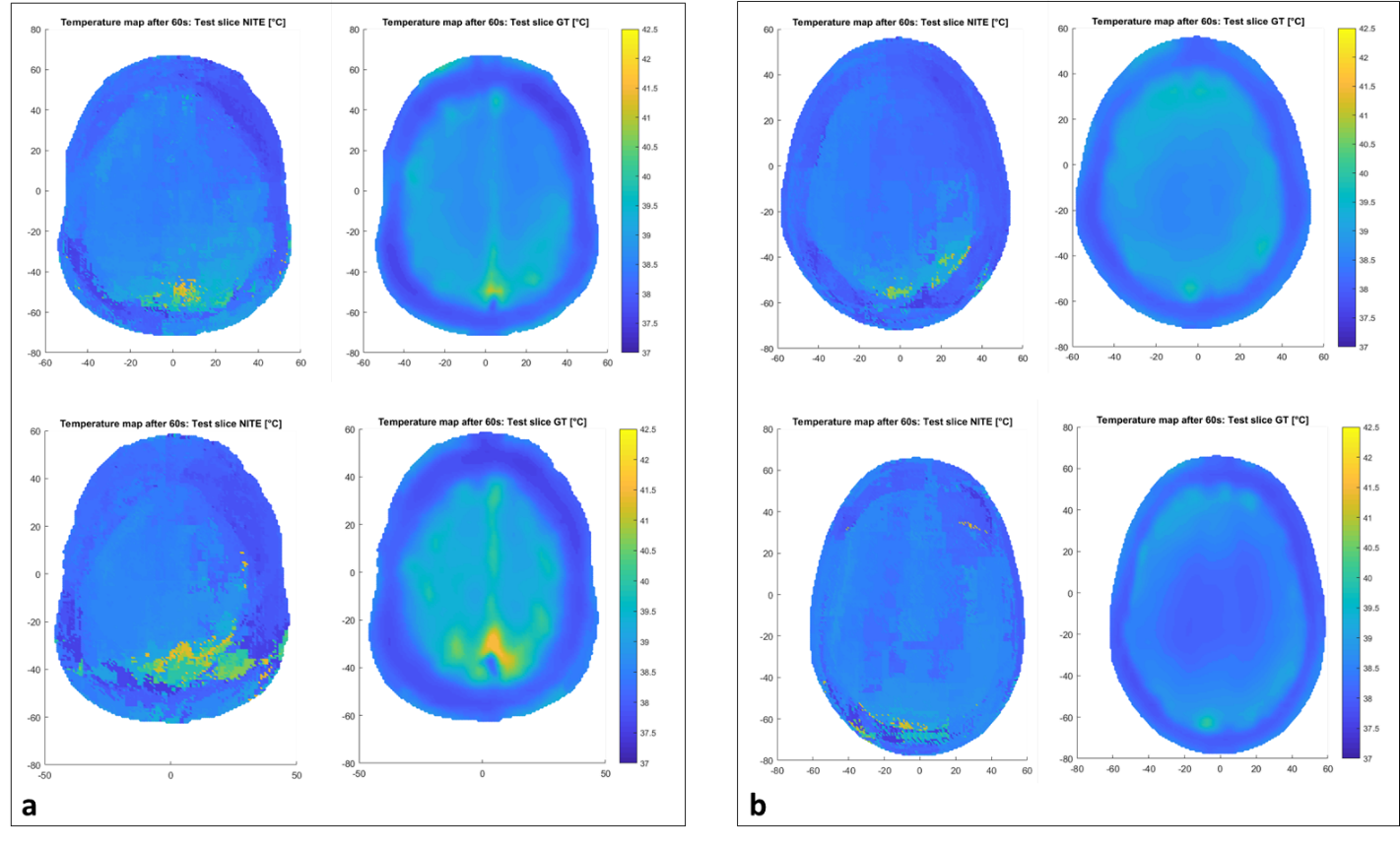
Figure 4: Temperature maps results. a. First and second row,
left: NITE-predicted temperature map on the first and second test slice
from HUGO’s brain (intra-brain testing). First
and second row, right: reference CST-simulated temperature map. b. Same results for NELLY’s first and
second test slices (inter-brain testing).

Figure 5: Quantitative comparison. a. First and second row, left: Temperature correlation between NITE
and CST for the first and second test slice from HUGO’s brain (intra-brain
testing). First and second row, right:
Difference-temperature maps for HUGO’s first and second brain slices. b. Same results for NELLY’s first and
second test slices (inter-brain testing).