4186
Modelling Static Field Induced Torque on Simplified Medical Devices
Xiao Fan Ding1, William B. Handler1, and Blaine A. Chronik1
1The xMR Labs, Department Physics and Astronomy, Western University, London, ON, Canada
1The xMR Labs, Department Physics and Astronomy, Western University, London, ON, Canada
Synopsis
The most recent published standard of static field induced torque on medical implants relies on solely experimental measurements. This study looks into the development of a computational method relying on the finite element method. It was found that for stainless steel rods, the percent difference between the numerical and measured torque values was less than 5%.
Introduction
The most recent test standard published in 2017 by ASTM International for assessing static field induced torque on medical implants outlined five experimental test methods [1]. This was an update to the first edition from 2006 which included one experimental method [1,2]. Currently, there are no internationally recognized methods for assessing torque by computational means. In the development of systematic and efficient testing of medical device safety, numerical methods based on the finite element method (FEM) are a possible tool that could be used to model the torque induced on devices placed in the static field environment of an MR scanner. A model was created in COMSOL (COMSOL Inc., Sweden), an FEM solver, to calculate torque on simplified devices, SS304 and SS316 cylindrical rods, and compared to experimental measurements, where the torque is measured using the pulley method outlined in ASTM F2213-17.Methods
The torque induced on sixteen cylindrical rods made of SS304 and SS316 (diameters of 0.64 and 1.27 cm and lengths of 3, 5, 7, and 9 cm) was measured on a 3 T scanner. Shown in Figure 1, the rods were placed on a 3D printed rotatable holder designed to fit both diameters. Connected to the holder was a spindle sitting atop a pointed wooden peg from which a thread was extended to a force gauge that was only capable of moving linearly. The apparatus with rods were positioned in the bore of the scanner such that the rods were exposed to the uniform static field at the center. While the rods were initially aligned with the static field, they were rotated away from alignment as the force gauge was pulled away slowly. The torque induced on the rods creates a measurable tension in the thread. After a full rotation, the peak force, F, was recorded and repeated without the rods to record the friction in the apparatus, Ff. Along with the known radius of the spindle, R, the torque, τ, can be calculated.$$\tau=R(F-F_f)$$In COMSOL, a simulation domain of a cylinder placed within a cube was created. The dimensions of the cylinders matched those of the machined rods for experimental verification. The cylinders were defined by the magnetic susceptibility, χ, while all other domains were defined as air and all objects were discretized with tetrahedra. Two physics solvers were used, Magnetic Fields, No Current and PDE Coefficient, to solve for B and ∇B respectively. A 3 T external field was applied, and the cylinders were rotated in the simulation domain, as the physical rods were rotated experimentally. The B, ∇B, and dV of each element were exported from COMSOL and used to calculate the force on each element using the following relation [3].
$$\mathbf{F}=\frac{\chi dV}{\mu_0(1+\chi)}\left(\begin{array}{rcl}(B_x\frac{\partial{B_x}}{\partial{x}}+B_y\frac{\partial{B_x}}{\partial{y}}+B_z\frac{\partial{B_x}}{\partial{z}})\mathbf{\hat{x}}\\(B_x\frac{\partial{B_y}}{\partial{x}}+B_y\frac{\partial{B_y}}{\partial{y}}+B_z\frac{\partial{B_y}}{\partial{z}})\mathbf{\hat{y}}\\(B_x\frac{\partial{B_z}}{\partial{x}}+B_y\frac{\partial{B_z}}{\partial{y}}+B_z\frac{\partial{B_z}}{\partial{z}})\mathbf{\hat{z}}\end{array}\right)$$The torque on each element at a distance, r, from the center of the cylinder was calculated given that τ=F×r. Summing up the torque on each element to get the net torque on the cylinder. The peak torque during the rotation in the simulation domain was then compared to the experimentally measured peak torque.
A parametric sweep of χ from 1E3 to 15E3 ppm was performed for the eight unique geometries. Using the equation of the linear fit between the simulated peak torques and χ2, the susceptibilities of every rod was calculated from the measured peak torques. As the rods of the same material and diameter were cut from the same initial piece of raw material, each set is expected to have the same/similar susceptibility. So, for each set of four rods, the mean susceptibility was calculated and used as the defining material property in COMSOL for the original piece of material.
Results
Figure 3 shows the linear plots of simulated peak torques against χ2 from the susceptibility sweep as well as the equation for the line of best fit between torque and χ2. The experimentally measured and simulated torques for each rod are tabulated Figure 4 which also includes the percent differences between numerical and measured values. The experimental values were used to calculate the susceptibility of each physical rod for which the mean of each set was calculated.Discussion and Conclusion
As expected, the numerical torque values were directly proportional to χ2. Both the experimental and numerical torque peaks in Figure 4 appear to increase linearly with length of the rod. The percent difference between the numerical and experimental values shown in Figure 4 were less than 5%. The susceptibilities calculated all lie in the range expected for the stainless-steel materials often reported as between 1000 to 20000 ppm with SS316 more precisely known to be between 3520 to 6700 ppm [4]. It is important to note that this method still requires validation using a material with known susceptibility. However, internally the simulation is seen to be self-consistent and given this self-consistency, FEM models would provide an effective tool to correctly identify the worst case amongst a family of devices, and so minimize the number of measurements to be performed experimentally to determine safety for a large group.Acknowledgements
The authors would like to acknowledge The Ontario Research Fund, NSERC, and the Canadian Foundation for Innovation.References
- ASTM International. (2017). Standard Test Method for Measurement of Magnetically Induced Torque on Medical Devices in the Magnetic Resonance Environment.
- Woods, T. O. (2007). Standards for Medical Devices in MRI : Present and Future. Journal of Magnetic Resonance Imaging, 26, 1186–1189. https://doi.org/10.1002/jmri.21140
- Nyenhuis, J. A., Park, S.-M., Kamondetdacha, R., Amjad, A., Shellock, F. G., & Rezai, A. R. (2005). MRI and Implanted Medical Devices: Basic Interactions With an Emphasis on Heating. IEEE Transactions on Device and Materials Reliability, 5(3), 467–480.
- Schenck, J. F. (1996). The role of magnetic susceptibility in magnetic resonance imaging: MRI magnetic compatibility of the first and second kinds. Medical Physics, 23(6), 815–850.
Figures

Figure 1: a) The rod holder and spindle sitting atop a pointed wooden peg b) The
holder with a d = 0.64 cm rod c) The holder with a d = 1.27 cm rod d) The force
gauge placed on a mechanism that allows for linear displacement, i.e. pulling
the thread. The force gauge was positioned as close to the scanner as allowed with
the thread under tension. As the force gauge is moved to the left, the rods
rotate e) The crank that operates the linear displacement mechanism
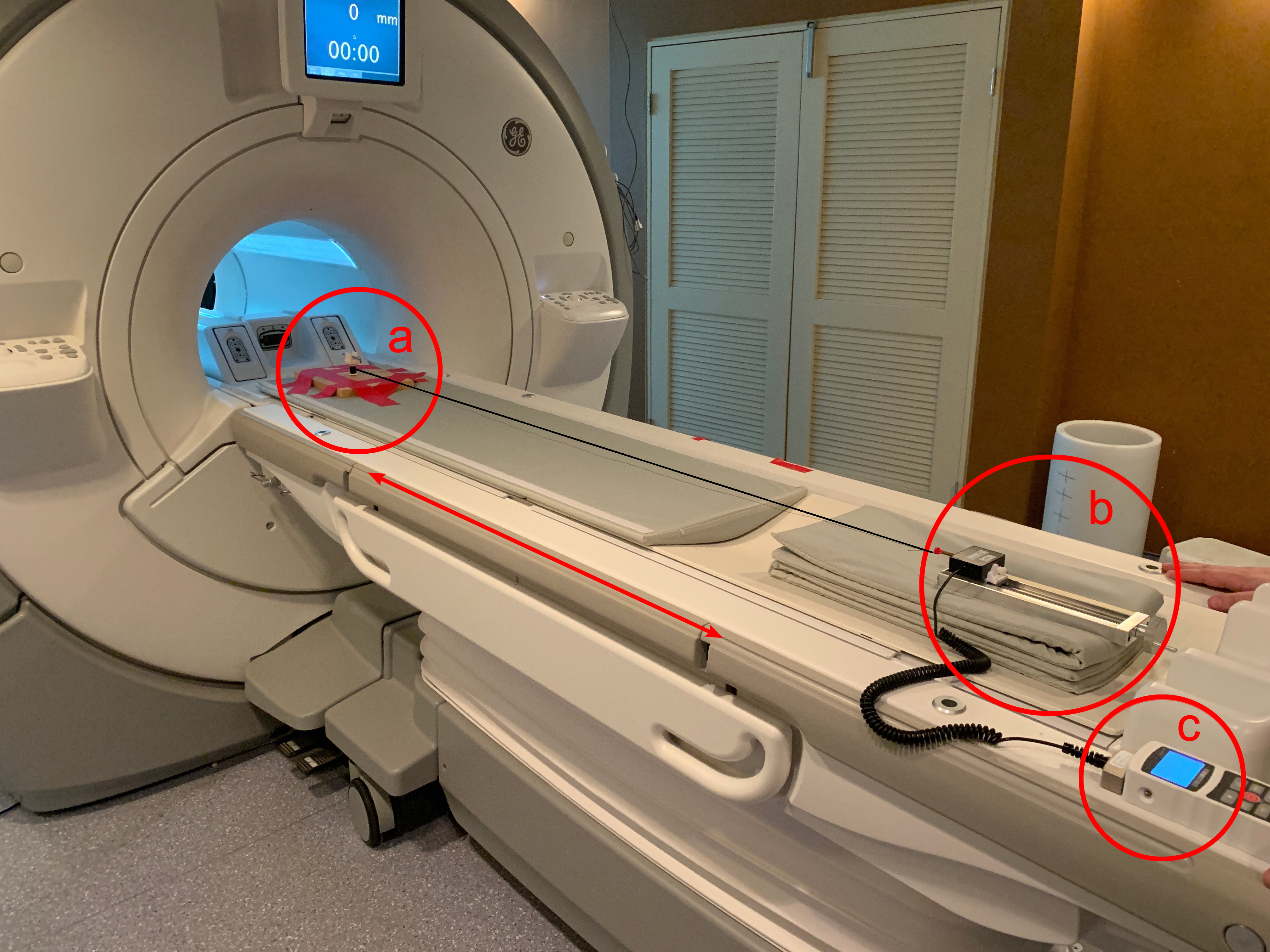
Figure 2: a) and b) are from Figure 1 and c) is the force gauge
display. The patient bed positions the rods into the isocenter. The rods were
aligned with the static field and the force gauge was slowly pulled away to
pivot the rods away from equilibrium. This resulted in an induced torque on the
rods to rotate back to equilibrium, which manifests as tension in the thread,
and is recorded by the force gauge. For each rod, the peak force during a full
rotation was used to calculate the peak torque.

Figure 3: There were sixteen rods in this study but only eight unique
geometries (d = 0.64 and 1.27 cm and l = 3, 5, 7, and 9 cm). Torque is seen to
vary with susceptibility squared but also with geometry. So, the eight linear
plots refer to the simulated peak torques for each unique geometry as the
susceptibility was varied from 1E3 to 15E3. The experimentally measured peak
torques were used to calculate the susceptibilities of the rods from the linear
equations.
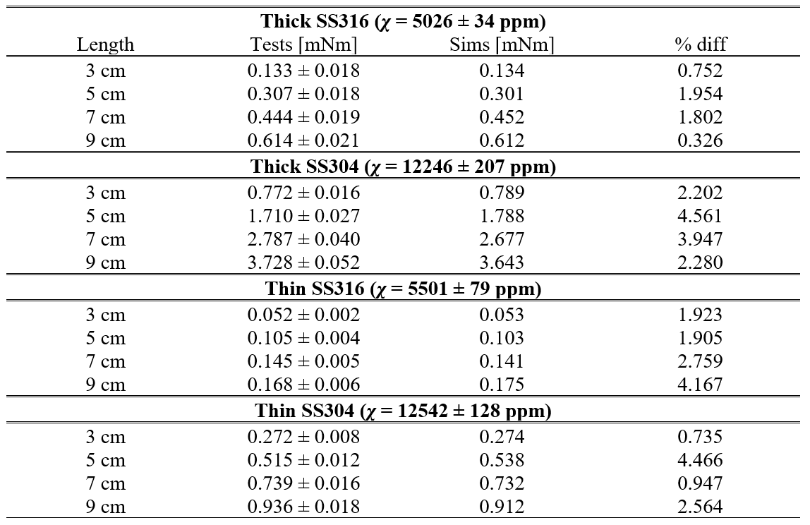
Figure 4: Using the mean susceptibility
calculated for each set of rods, the simulated torques were calculated and
compared to measurement. This comparison gives us a sense of the numerical
accuracy. The percent difference between numerical and experimental is always
less than 5%.