Introduction

MRI provides for diverse tissue contrasts through different pulse sequences. Each sequence involves multiple configurable parameters that need optimizing for contrast, acquisition time and signal-to-noise ratio. However, a large number of combinations exist (for example, 29 million for 12 protocols (1)) and choosing an optimal combination in real-time is difficult. Previous work involved analytically solving the signal models to derive optimal combinations (2), or populating a LUT with values derived from analytical models (3). These methods are computationally intensive and do not scale easily. In this work, intelligent protocolling is performed by leveraging a LUT populated by data collected from a vendor’s simulator. Intelligent protocolling can be leveraged to maximise MR Value, which can be loosely defined as the ratio of image contrast to acquisition time.

Methods

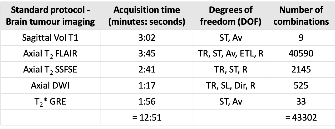
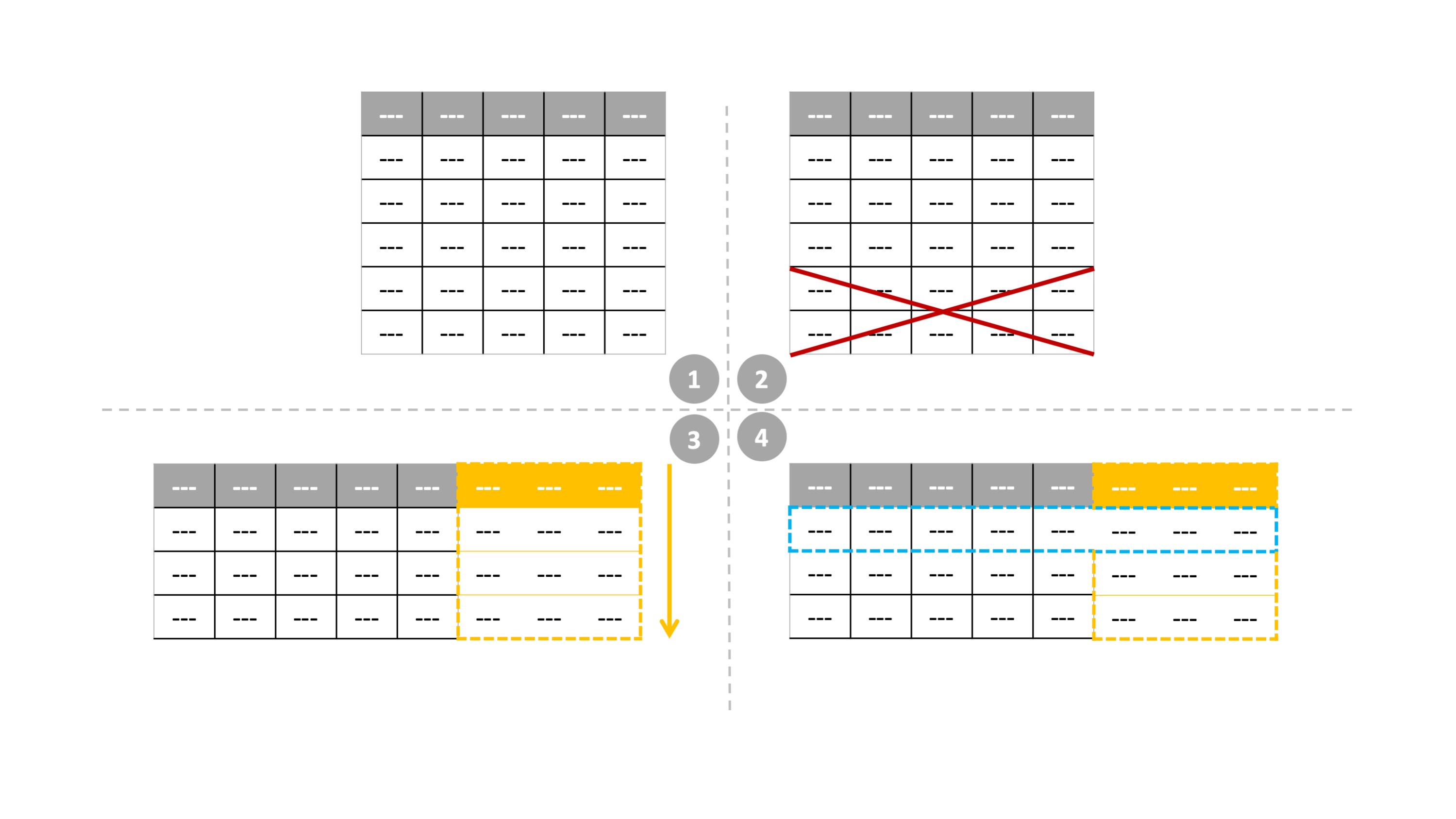
This work involves consulting LUTs to perform intelligent protocol optimization to meet an acquisition time constraint. The non-contrast brain tumor imaging protocol utilized routinely at our institution was held as the control protocol in this work, and is referred to as the ‘standard protocol’. The standard protocol’s acquisition time was 12:51 (minutes: seconds). For each pulse sequence in the standard protocol, specific sequence parameters (degrees of freedom, DOF in Table 1) that could be modified while not deviating from the image contrasts were chosen. The corresponding ranges of values were noted and exhaustive combinations of relevant DOF were generated for each sequence. The LUT was populated by recording relative SNR (rSNR) and acquisition time from a vendor’s simulator for all or hundred randomly chosen combinations, whichever was smaller. A regression fit was performed to compute the time allocation as a percentage of the protocol time constraint. The LUT search algorithm (Figure 1) was designed to discard parameter combinations that did not meet this time constraint. Then, a final score was computed as the weighted sum of deviations of each DOF from the corresponding values in the standard sequences. Finally, the parameter combination with the lowest score was chosen. The LUTs for the remaining sequences were constructed and searched similarly. Parameters that affect image contrast and slice thickness were assigned larger penalties while rSNR was assigned a smaller weight. The minimum overall acquisition time obtained from the LUTs was 4:56 (minutes: seconds). Four experiments were performed to acquire in vivo data from a healthy volunteer (IRB approved study). The standard protocol and three modified protocols obtained from LUTs for 5:00, 7:30, and 10:00 time constraints were executed. The data were acquired on a GE Discovery 750w scanner. Quantitative analysis involved comparing the LUT rSNR versus measured rSNR. For the measured rSNR, brain matter signal intensities were averaged after masking the background using a threshold. For sagittal T1 volume, a region-of-interest mask was hand-drawn. The standard deviation of a 20x20 corner patch from the top-left region of the image was computed to obtain the noise value. Then, SNR (dB) was computed as the ratio of mean signal intensity to noise. Finally, rSNR was obtained by calculating the SNR values for the modified protocols as a percentage of the SNR values from the standard protocol.

Results

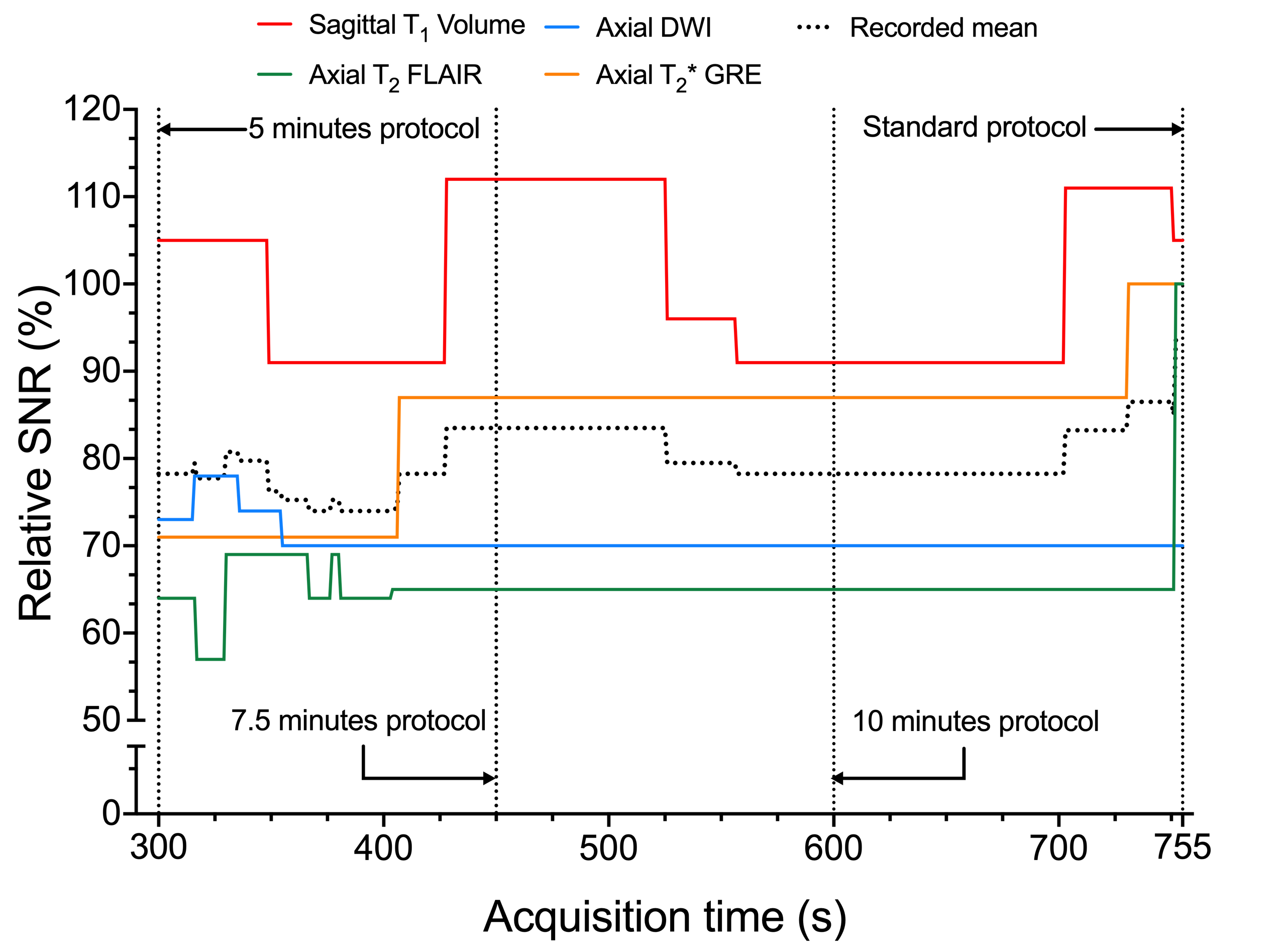
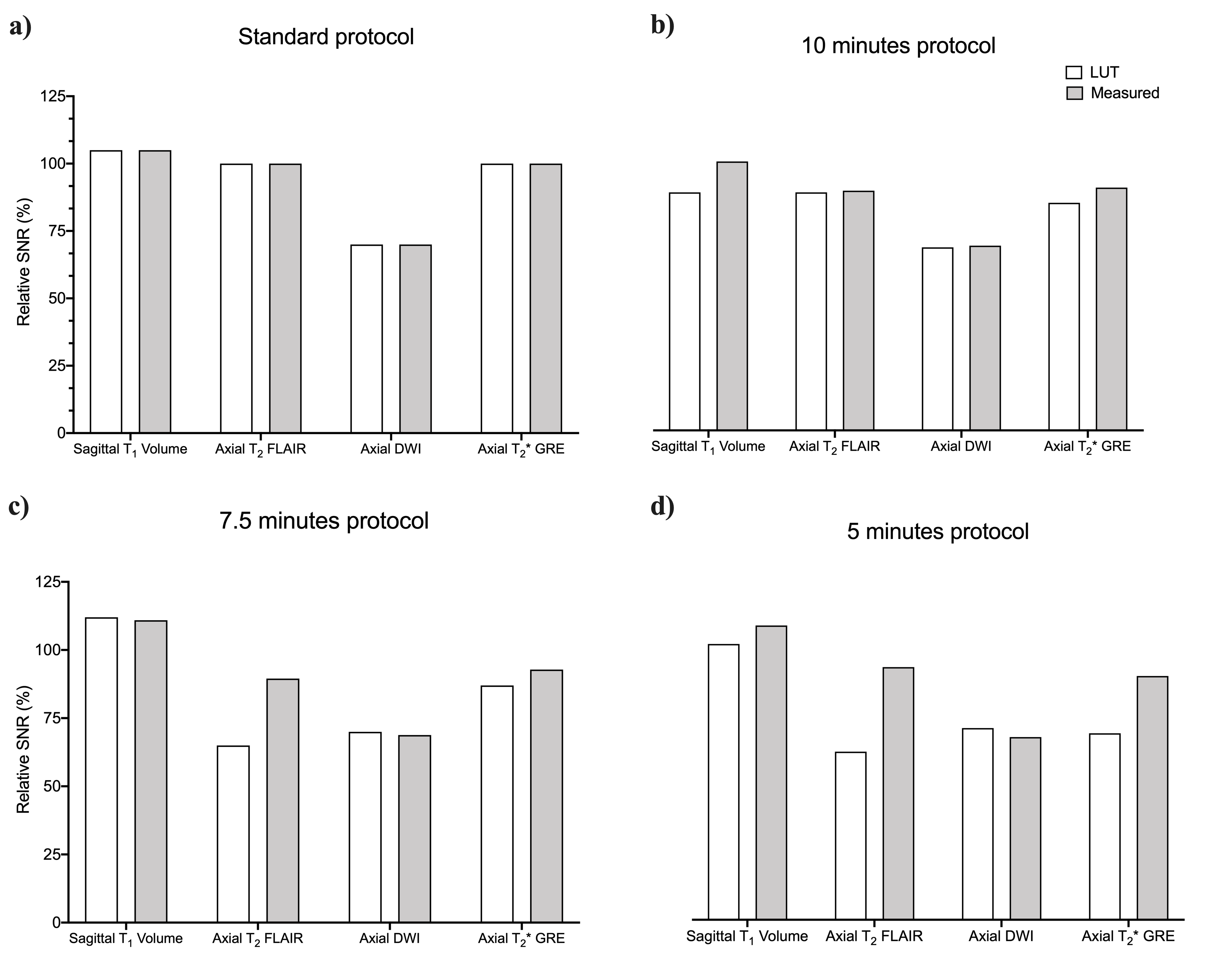
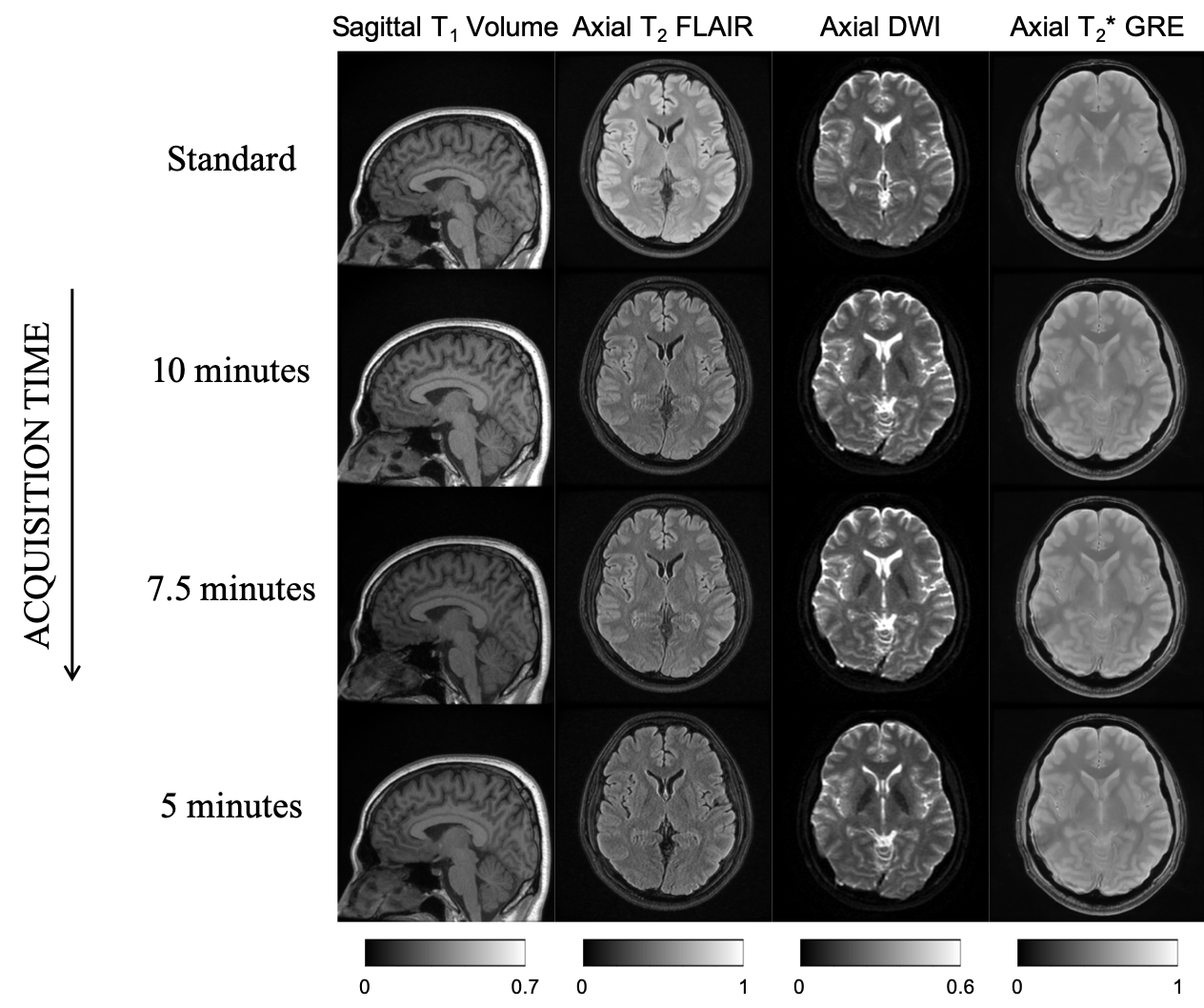
Table 1 describes the standard protocol employed at our center. Overall, there were 43,302 combinations across all DOF. Figure 2 is a graph of rSNR values obtained from the LUT over a range of acquisition time constraints. The rSNR values for the 5 minute protocol versus the standard protocol as per the LUT is 78.25% versus 93.75% and % versus 92.5% as per the acquired data . Figure 3 compares LUT- and measured-rSNR values across the four experiments. Values for axial T₂ using SSFSE are not reported because the data was motion corrupted. Figure 4 shows the single-slice reconstructions from the four experiments. Qualitatively, image contrasts of the three modified protocols have not deviated significantly from that of the standard protocol.

Discussion

Based on inputs from a radiologist and MR technician, DOF for each sequence were chosen such that the modified protocol’s image contrast was not significantly different from the standard protocol’s image contrast. SNR was allowed to be compromised as SNR is recoverable post-acquisition by deep learning methods (4, 5). Future work involves automating data collection by leveraging existing vendor-provided or third-party tools. The resulting variable space will be larger and require more robust search techniques for the LUT operation. Further validation of the LUT by acquiring data from a larger number of volunteers is necessary. Subsequently, the LUT can be integrated into Autonomous MRI’s workflow (3).

Conclusion

Three modified protocols were derived from the standard protocol for 5:00, 7:30 and 10:00 time constraints. A 7:55 (minutes: seconds) decrease in acquisition time resulted in a 15.5% drop in SNR. Qualitative image contrast was maintained across the four sequences (Figure 4). The LUT enabled searching higher-dimensional spaces. This potentially allows gathering insights about protocol optimisation that would otherwise not be straightforward due to the number of acquisition parameter combinations possible.

References

1. Block, Tobias, et al. “Creating New Value Through Innovation.” ISMRM-RSNA Co-Provided Workshop on High-Value MRI, Washington D.C., USA (2018).
2. Soltanian-Zadeh, Hamid, et al. "Optimization of MRI protocols and pulse sequence parameters for eigenimage filtering." IEEE transactions on medical imaging 13.1 (1994): 161-175.
3. Ravi, Keerthi Sravan et al. “MR Value driven Autonomous MRI using imr-framework”. ISMRM Workshop on Machine Learning Part II, Washington D.C., USA (2018).
4. Chaudhari, Akshay S., et al. "Super‐resolution musculoskeletal MRI using deep learning." Magnetic resonance in medicine 80.5 (2018): 2139-2154.
5. Benou, Ariel, et al. "De-noising of contrast-enhanced MRI sequences by an ensemble of expert deep neural networks." Deep Learning and Data Labeling for Medical Applications. Springer, Cham, 2016. 95-110.