4031
Development of a biplanar volume coil for an open 0.1 T MRI system1Laboratory for Adaptable MRI Technology (AMT lab), Dpt of Biomedical Engineering, University of Basel, Allschwil, Switzerland, 2Medical Image Analysis Center (MIAC AG), Basel, Switzerland
Synopsis
An open, biplanar volume RF coil was built and tested as a transceiver with a homogeneous B1 at 4.2 MHz. We demonstrate its feasibility and performance in a low-field, open biplanar magnet. While giving good sensitivity, this geometry provides easy access to the object from multiple sides. In addition to simpler positioning of patients, this potentially opens the way for improved MRI applications where access is primarily required such as interventional MRI.
Introduction
Many low-field MRI systems employ open biplanar magnets, combining the advantages of the low field with an enhanced access to the patient. The most common volume RF coils used in these magnets, such as solenoids or Helmholtz coils, provide increased homogeneity and coverage, yet they do not provide open access to the imaged sample from all available sides1. Surface coils, on the other hand, provide good access to the sample with high sensitivity, but at the cost of poor coverage.Here, a custom biplanar coil that combines high homogeneity and coverage while maintaining open access to the sample is proposed for a 0.1 T biplanar vertical magnet, based on previous work at 1.5 T2. Such a coil provides access from all the three open sides of our magnet while maintaining a high filling factor due to close proximity with the object for SNR improvement3.
Methods
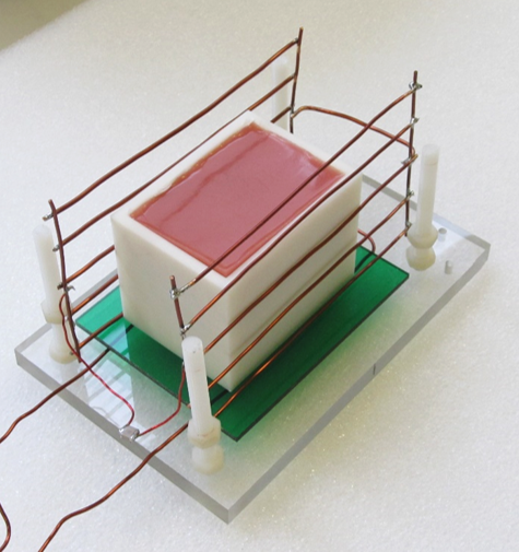
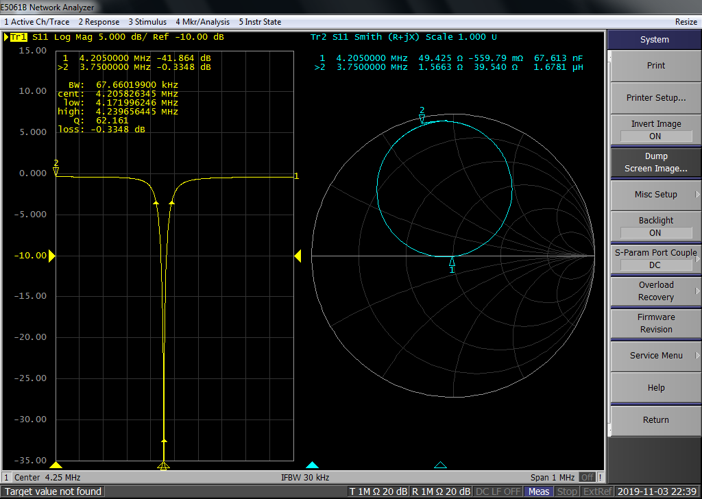
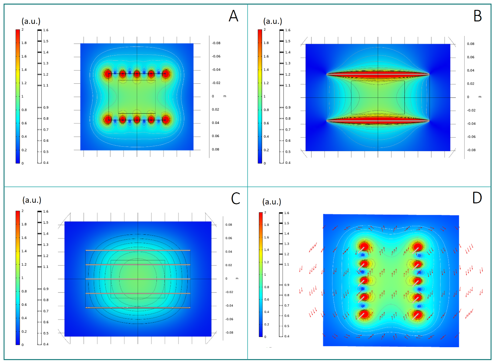
Simulations of the coil’s B1 field were done using the AC/DC module of COMSOL Multiphysics© (COMSOL AB, Sweden). The wires connecting the parallel segments were neglected and a unitary AC current was imposed in input/output of the latter.The coil (Fig 1) was built using segments of solid copper wire of Ø 1.6 mm. Both sides are composed of 5 equally spaced straight rods soldered in parallel. Both planes are 15.5 x 8.5 cm2 in size, separated by 7 cm and connected by copper wire to ensure proper current flow direction. The coil was tuned using a single 5.74 nF capacitor and inductively matched to 50 Ω (Fig 2) with a copper loop4.
MRI was performed at 0.1 T on a resistive biplanar magnet (Bouhnik S.A.S., France), with the coil interfaced in transceive mode using a commercial TR switch (NMR Service GmbH, Germany) and a custom preamplifier.
Raw signals were acquired with a Cameleon 3 spectrometer (RS2D, France) using a custom, spoiled 3D GE sequence with the following parameters: acq. matrix 44 x 31 x 9, voxel size 2.1 x 2.8 x 7.8 mm3, TE/TR 4.13/23 ms, and NA 100. A variable density gaussian undersampling pattern of 60% was used in the phase-encoding of k-space, leading to a total acquisition time of 6 min and 24 s. Image reconstruction was performed using MATLAB (Mathworks, USA). A rectangular silicone phantom, of the size of the simulated volume of interest was used as a specimen, with the second phase-encoding direction parallel to B1.
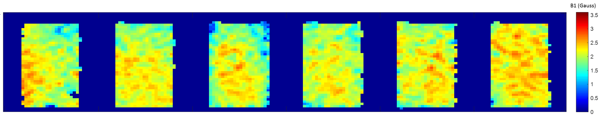
B1 maps were obtained from a double-angle approach with two images at respectively 45° and 90° nominal flip angles. The flip angle was changed by varying the duration of a rectangular excitation pulse while keeping its amplitude constant. The images were pre-filtered with a Tukey window (cosine fraction 0.8).
Results
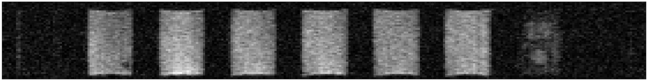
The simulations show that the chosen coil geometry and number of wires provide good B1 homogeneity within a volume of interest of 8 x 5.6 x 5 cm3 (Fig 3). Besides, the orientation of B1 field (Fig 3d) shows that the coil grids can be positioned parallel to the main B0 coils of our biplanar magnet, with minimal space obstruction.The assembled coil was properly tuned and matched by adjusting the position of the coupling loop (Fig 2). Images obtained at 4.2 MHz are presented in Fig 4, with an average SNR of 16 across the object. The obtained B1 maps (Fig 5) show good homogeneity within the imaged volume. An improvement of +9% in SNR could be obtained by adding a very simple shielding consisting of two Cu-FR4 plates on the two sides of the coil.
Discussion
Our RF coil used in transmit and receive produced images at 0.1 T with a homogeneous signal in the volume of interest. The expected homogeneous B1 distribution was verified experimentally, confirming the simulations. However, the coil can be further optimized in terms of geometrical parameters and size of copper wire. Larger versions will be investigated for more efficient use of our biplanar magnet’s inner space. Partial shielding of the coil can be easily implemented without impeding access.Conclusions
An open, biplanar volume RF coil was simulated, built, and successfully tested at 4.2 MHz that provides high homogeneity and sensitivity. We aim to optimize its design depending on envisioned applications, for enhanced access and sensitivity in diverse sample sizes.Acknowledgements
No acknowledgement found.References
1. Mispelter J and Lupu M. 2008 “Homogeneous Resonators for Magnetic Resonance: A Review.” Comptes Rendus Chimie 11 (4–5): 340–55.
2. Roberts DA, Insko EK, Bolinger L, et al. 1993. “Biplanar Radiofrequency Coil Design.” Journal of Magnetic Resonance, Series A 102 (1): 34–41.
3. Blasiak B, Volotovskyy V, Deng C, et al. 2009. “An Optimized Solenoidal Head Radiofrequency Coil for Low-Field Magnetic Resonance Imaging.” Magnetic Resonance Imaging 27 (9): 1302–8.
4. Hoult DI and Tomanek B. 2002. “Use of Mutually Inductive Coupling in Probe Design.” Concepts in Magnetic Resonance Part B: Magnetic Resonance Engineering 15 (4): 262–85.
Figures