4023
Dipole Decoupling with Parasites1Medical Physics in Radiology, German Cancer Research Center (DKFZ), Heidelberg, Germany, 2Physics & Astronomy, Heidelberg University, Heidelberg, Germany
Synopsis
We investigate the decoupling of a pair of fractionated dipoles using an additional passive parasitic dipole. Decoupling is optimised either geometrically, by adjusting the parasite length and standoff distance from the active dipoles, or by adding resistance and reactance to the parasite centre. Adjusting two parameters allows control over the amplitude and phase of the decoupling signal induced via the parasite, producing very strong decoupling at the target frequency (better than -40 dB). The effect is demonstrated using EM simulation and verified with bench measurements.
Introduction
Dipole antennas have become popular transmit elements for UHF MRI, largely due to their high efficiency in generating B1 field deep inside a sample [1]. However, decoupling of dipoles in an array remains an outstanding problem, with most decoupling techniques used for conventional loop array being difficult to translate for use with dipoles.The problem of decoupling antennas arranged in close proximity is well known in the antenna design world, particularly for MIMO (multiple-input-multiple-output) antenna design [2,3]. One popular approach is the use of parasitic elements - i.e. non-driven antennas, used to introduce an additional coupling pathway to cancel the problematic coupling. This approach has been previously applied to array coil design for MRI [4], introduced as ICE decoupling. However, in assuming purely reactive decoupling, the optimal decoupling point was not found.
In this abstract we investigate decoupling of two fractionated dipoles by adding a parasitic dipole. Decoupling is optimised either purely geometrically, or by adding resistive and reactive components to the centre of the parasite. By controlling two components, we achieve very strong decoupling between neighbouring elements.
Methods
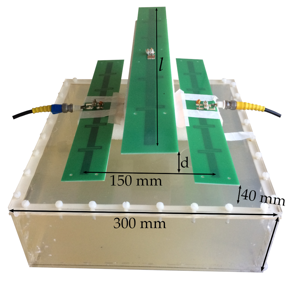
Two fractionated dipoles using the dimensions given in [1], and a passive fractionated parasitic dipole, were simulated in front of a homogeneous cuboid phantom (εr = 34, σ = 0.4 S/m) using CST Studio Suite 2019 (Dassault Systèmes). Bench measurements were made using dipoles and parasites constructed from 1.55mm FR4 boards using 35 µm copper. Loading was provided by a 300×300×100 mm3 agar phantom, doped with sugar and salt to give εr = 53.7 and σ = 0.68 S/m [3]. Coupling measurements were made between the dipoles in the presence of various parasites using a network analyser (E5061B, Agilent). In simulation and experiment, the dipole antennas were placed 40 mm away from the phantom and separated by 150 mm (figure 1). Both dipoles were tuned to 297 MHz and matched to better than -30 dB. The parasite length $$$\ell$$$, stand-off distance $$$d$$$, and additional resistance $$$R$$$ and capacitance $$$C$$$ were then varied to minimise coupling between the active dipoles.Results
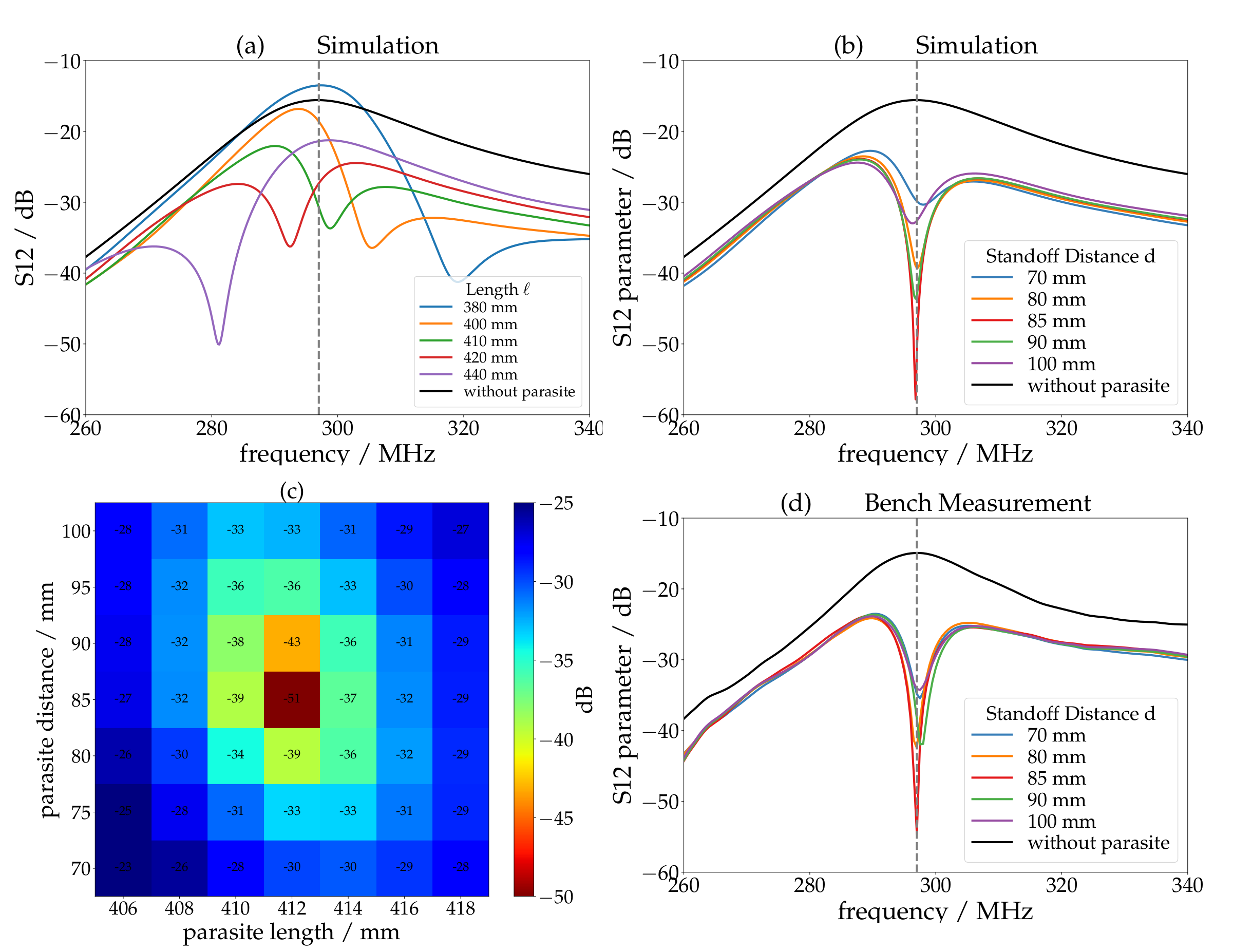
Figure 2a shows simulated coupling between two dipoles. The black curve shows the coupling when no parasite is present, while remaining curves illustrate the coupling when a parasite of length 380-440mm was added, at a fixed standoff distance of 75mm from the plane of the dipoles. The parasite created a strong local minimum (< -30dB) in the coupling between dipoles. Changing the parasite length shifts the frequency of the minimum. Figure 2b shows the influence of adjusting the parasite standoff distance from the dipole plane, which affects the depth of the decoupling minimum while having almost no influence on the resonance frequency ($$$\ell$$$ = 412 mm). Figure 2c shows the coupling between dipoles as the parasite length and standoff distance were swept, showing optimum decoupling at $$$\ell$$$ = 412 mm and $$$d$$$ = 85 mm. Figure 2d shows the experimental verification of the simulation results shown in figure 2b, measured using the setup shown in figure 1. The standoff distance $$$d$$$ was then reduced to 20 mm, and coupling investigated as a function of resistance and capacitance added to the centre of the parasite. Figure 3a shows a sweep over resistance and capacitance, with a strongest minimum at $$$C$$$ = 26 pF and $$$R$$$ = 18 Ω. Figure 3b compares simulated (blue) and measured (red) coupling.Discussion and Conclusions
Neighbouring dipoles can be decoupled by adding a parasitic dipole between them. Strong decoupling requires control over the amplitude and phase of the additional coupling signal induced by the parasite (this approach is similar to [6]). This can be achieved geometrically, by adjusting the length of the parasite and it's standoff distance from the dipoles, or by adding a resistive and reactive load to the parasite centre. Using purely geometric adjustment resulted in parasites slightly longer than the active dipoles (412 vs. 300 mm), and a standoff distance of 85mm. As space is typically limited inside the magnet bore, use of a smaller standoff distance is attractive, although it should not be so small that the parasites affect the $$$B_1^+$$$ or $$$E$$$ fields inside the sample. For a standoff distance of 20 mm, coupling was minimised by adding a loading of $$$R$$$ = 18 Ω and $$$C$$$ = 26 pF in simulation, and $$$R$$$ = 6 Ω and $$$C$$$ = 7 pF when measured at the bench. Differences between simulated and measured values are thought to be due to differences in loading between the two setups. In both cases, decoupling of better than -40 dB was easily achieved.It is interesting to compare our results to those in [7], where it was reported that decoupling effectiveness decreased when the parasitic elements were moved away from the load. A strong local coupling minima is actually visible in those results, but it was not 'tuned' to the desired operating frequency, demonstrating the importance of controlling the resonance frequency of, and degree of coupling to, the parasite.
To fully demonstrate the parasite decoupling method, we are now building an 8-channel dipole array, including six parasites for decoupling, for imaging the kidney and pelvis regions in the human body at 7T.
Acknowledgements
No acknowledgement found.References
[1] Raaijmakers et al. MRM, 75(3), 2016; [2] Mak et al. IEEE Trans. Antennas Propag., 56, 2008; [3] Kalis et al, Parasitic Antenna Arrays for Wireless MIMO Systems, 2013; [4] Li et al, Med. Phys. 38(7), 2011; [5] Duan et al. Medical Physics, 41(10), 2014; [6] Avdievitch et al, NMR Biomed. 26(11), 2013; [7] Yan et al, MRI 34(9), 2016.
Figures
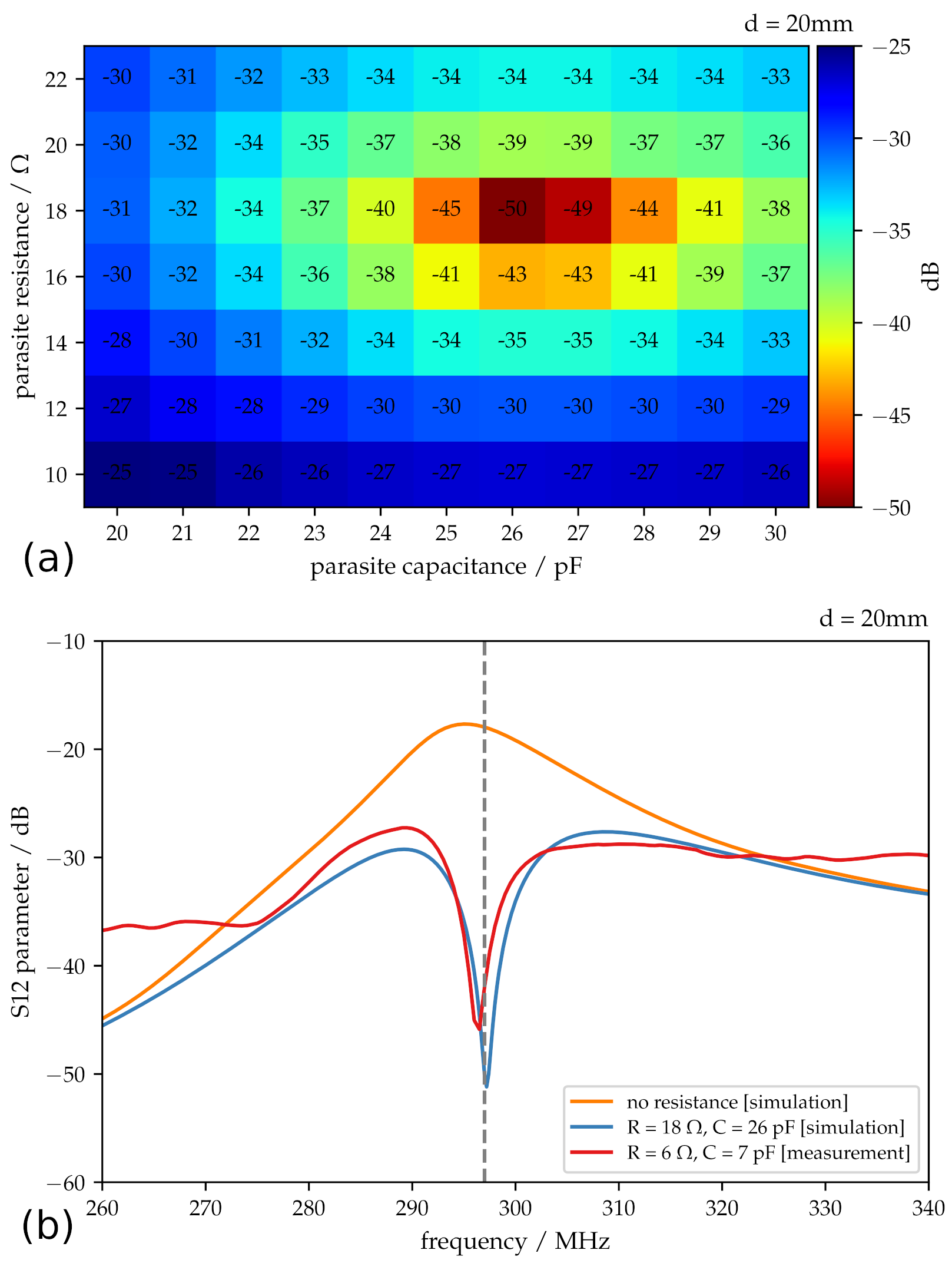
Coupling between dipoles (a) while sweeping over the parasite’s capacitance and resistance and (b) bench verification of simulation result.