4017
BOLD signal simulation and fMRI quality control base on an active phantom: a preliminary study1Medical Engineering and Technology Research Center, Shandong First Medical University & Shandong Academy of Medical Sciences, Taian, China, 2Shandong First Medical University & Shandong Academy of Medical Sciences, Taian, China, 3Shandong University of Science and Technology, Qingdao, China, 4Hubei Cancer Hospital, Tongji Medical College, Huazhong University of Science and Technology, Wuhan, China
Synopsis
The purpose of this study was to design and manufacture an active BOLD simulation phantom, thus testing the stability and repeatability of the phantom. Three scanners were used to test the stability and repeatability of the BOLD signal detection of the phantom. It was found that the phantom had good stability and repeatability. The phantom can stably quantify the BOLD signal for fMRI quality control in different scanners. Consequently, the phantom can stably quantify the BOLD signal for fMRI quality control in different scanners.
Introduction
The amplitude of the BOLD signal on the T2* images varies by approximately 1%-3% [1, 2]. Such a change in signal amplitude is expected to be very small compared to the imaging signal generated by the brain tissue. The MR scanner device can influence signal detection by field intensity, gradient, sequence design, and data processing protocol etc. It also affect by breathing, heartbeat, and head movement [3, 4]. Therefore, it is important for the quality control (QC) of fMRI and quantitatively measurement of BOLD signal detection efficiency. The phantom of Friedman et al. can be used to evaluate various static characters of scanner, such as SNR, noise etc., but it cannot achieve task-state stimulation [8]. Two liquids with slight differences in T1, T2 and T2* were used in Olsrud et al study to mimic the control and activation states of the brain. However, it is inconvenient because the "control part" and "activation part" should be moved manually to the coil center to switch two states [5]. Renvall et al. used the current-induced magnetic field to change the local magnetic field (B0) near the conductor. The advantage is that the signal changes can be synchronized with fMRI experiments easily. However, their phantom had a small area for analysis and was susceptible to heterogeneity of magnetic field [6]. In this study, a BOLD signal simulation phantom was manufactured, which can assist in three expected goals. Firstly, it is a basic function that can simulate BOLD signals, and quantitatively measure SNR, SFNR and ghost signal ratio etc.. Second, it is the simulation effect that can contribute to the completion of the module design, including adjustable stimulus size and duration. Furthermore, it is a repeatability assessment that can be applied to different conventional scanners for signal detection efficiency and percent signal change (PSC) evaluation.Methods
The phantom was fabricated by 3D printer using acrylonitrile butadiene styrene (ABS) material with fused deposition printing technique. Then, the agarose gel (31.5 g of agarose powder, 21.0 g of sodium chloride, and 4.2 ml of gadolinium diethylene-trianmine pentaacetic acid (Gd-DTPA) dissolved in 2100 ml of water) was poured into the phantom and stored in a package. Based on the micro control system 51 series (MCS 51), a stimulation circuit was designed for outputting square pulse. The circuit was placed outside the shield room and connected to the phantom in the dedicated head-neck coil via a copper wire. The fMRI simulation design: baseline (power off), active state . The same protocols were performed twice. Then data analysis processing was carried on Matlab 2013b (The MathWorks, Inc., Natick, MA, USA).Results
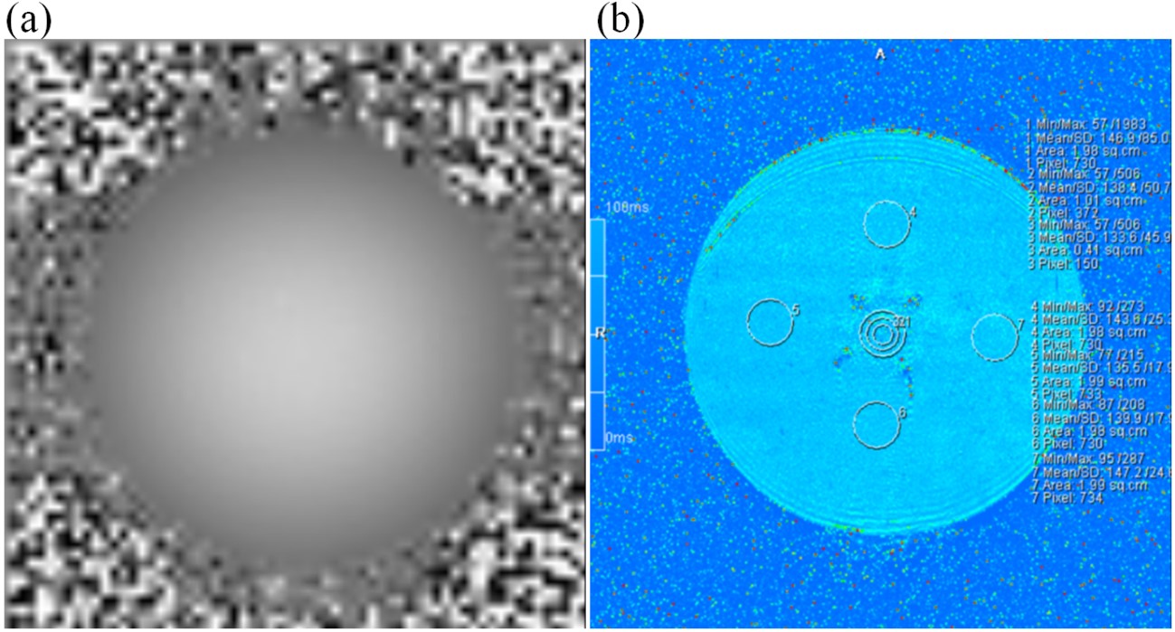
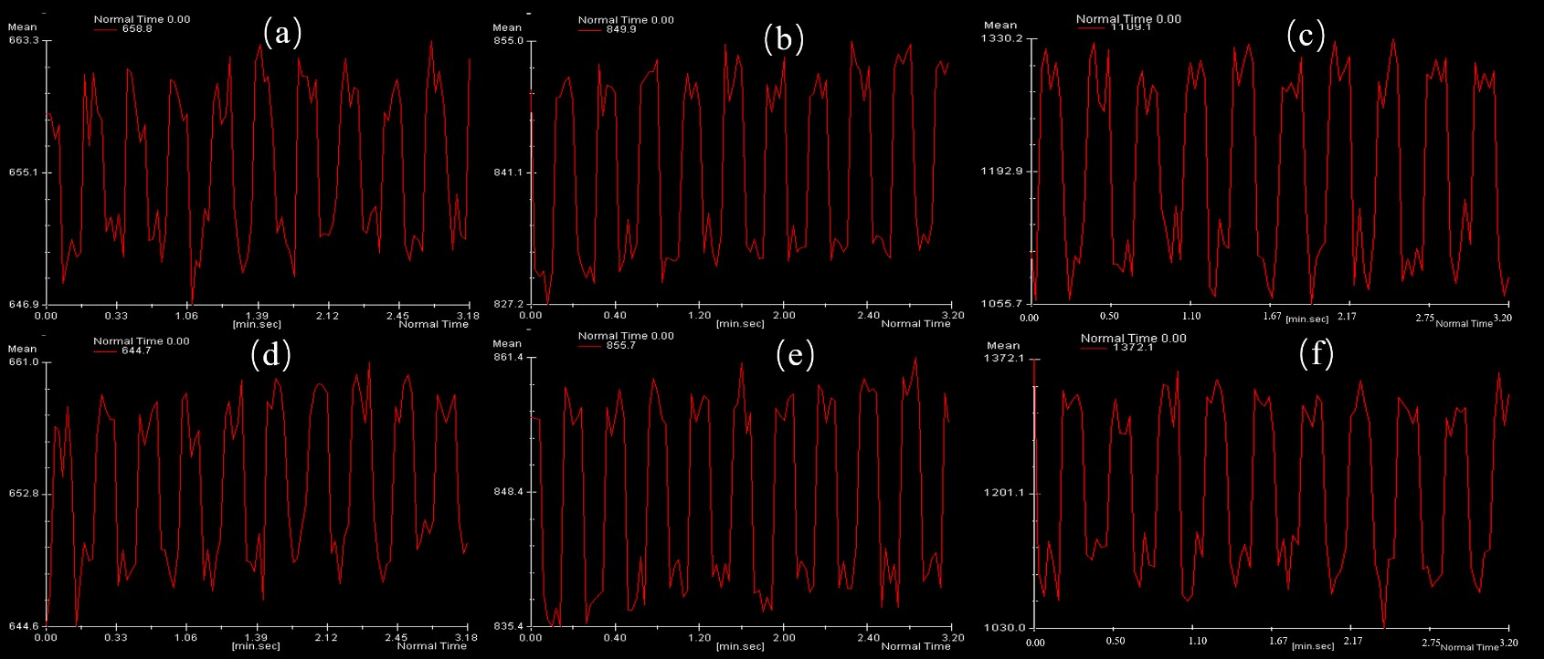
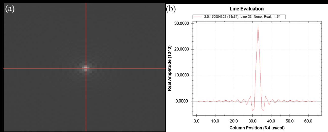
The signal distribution in the phantom was clearly observed in Fig 1, while the T1, T2, and T2* values of the central and peripheral regions in the phantom were displayed in Table 1. As shown in Fig 2 and Table 2, the signal in the central region was quite stable, with the average signal strength varies within 1%, and the variation range of signal values was less than 10. Fig 3 demonstrated a time-signal intensity curve for 24 mA current in the same ROI. The percent signal change (PSC) increased with the current level among three scanners (Table 3). The protocol on the same scanner was repeated to compute the number of effective stimuli per 100 scanning. All three scanners exhibited good repeatability. Here, the results of Simens Skyra 3.0T were shown in Fig 3. As displayed in Fig 4, the k-space was then obtained by choosing images at different time points, where no abnormally high noise was found. The raw data was subjected to slice timing and head motion correction using SPM, and t-map in the intermediate slice of the phantom was obtained through GLM analysis, as shown in Fig 5.Discussion
Conventional passive fMRI phantoms usually used different concentrations of the same material, causing differences in T1 and T2 relaxation times to simulate the BOLD signal variations [5, 6]. Manual operation in these phantoms is required, leading to an increased in the number of experimental variables. Compared to the Smartphantom [7], the area available for analysis in our phantom became larger, and our system could preferably match with different scanners. Moreover, the duration and intensity of the stimulus could be accurately adjusted to obtain the optimal stimulus scheme.Conclusion
The phantom was designed to stimulate the BOLD signal and fMRI QC, and the signal could be quantitative measured with stability and consistency.Acknowledgements
We would like to thank Yaoyao He, Fenglian Zheng, Haozhao Zhang, Xiaojing Liu and Shitong Zhang for their comments and suggestions.References
1. Jellinger KA. Clinical Applications of Functional Brain MRI. European Journal of Neurology. 2010;16(4):e86-e.
2. Liau J, Liu TT. Inter-subject variability in hypercapnic normalization of the BOLD fMRI response. Neuroimage. 2009;45(2):420-30.
3. Eklund A, Nichols TE, Knutsson H. Cluster failure: Why fMRI inferences for spatial extent have inflated false-positive rates. Proc Natl Acad Sci U S A. 2016;113(28):7900-5.
4. Leontiev O, Buxton RB. Reproducibility of BOLD, perfusion, and CMRO measurements with calibrated-BOLD fMRI. Neuroimage. 2007;35(1):175-84.
5. Friedman L, Glover GH. Report on a multicenter fMRI quality assurance protocol. Journal of Magnetic Resonance Imaging. 2010;23(6):827-39.
6. Olsrud J, Nilsson A, Mannfolk P, Waites A, Ståhlberg F. A two-compartment gel phantom for optimization and quality assurance in clinical BOLD fMRI. Magnetic Resonance Imaging. 2008;26(2):279-86.
7. Renvall V, Joensuu R, Hari R. Functional phantom for fMRI: a feasibility study. Magnetic Resonance Imaging. 2006;24(3):315-20.
8. Tovar DA, Wang Z, Rajan SS. A Rotational Cylindrical fMRI Phantom for Image Quality Control. Plos One. 2015;10(12):e0143172.
9. Cheng H, Zhao Q, Duensing GR, Edelstein WA, Spencer D, Browne N, et al. SmartPhantom — an fMRI simulator. Magnetic Resonance Imaging. 2006;24(3):301-13.
Figures