Introduction

Denoising task-based fMRI data is important for increasing SNR and has implications for data interpretation.¹ Researchers currently denoise task-based fMRI data through a variety of different methods, commonly by including experimental confounds that assess motion-related² or physiological noise³ as part of a first-level GLM. With so many different possible combinations of confounds, it can be difficult for novice researchers to determine the optimal course of action for de-noising a particular data set. There is not currently a method or tool available for directly comparing the relative impact of including different confounds (e.g., DVARS vs. framewise displacement) in a GLM. However, such a tool could provide researchers with valuable information to assist in deciding the most appropriate set of confounds to use for a given data set in order to maximize detection of the BOLD signal. Here we describe a new BIDS/fMRIPrep app, confounder, developed for these purposes, which utilizes the confounds.tsv output file from fMRIPrep⁴ – a field-supported standard and transparent method of fMRI data preprocessing. This tool as provides estimates of GLM model fit⁵ along with metrics, such as the correlation between experimental confounds and predicted BOLD signal of explanatory variables, to help researchers determine which confounds are most appropriately used for their data.

Methods

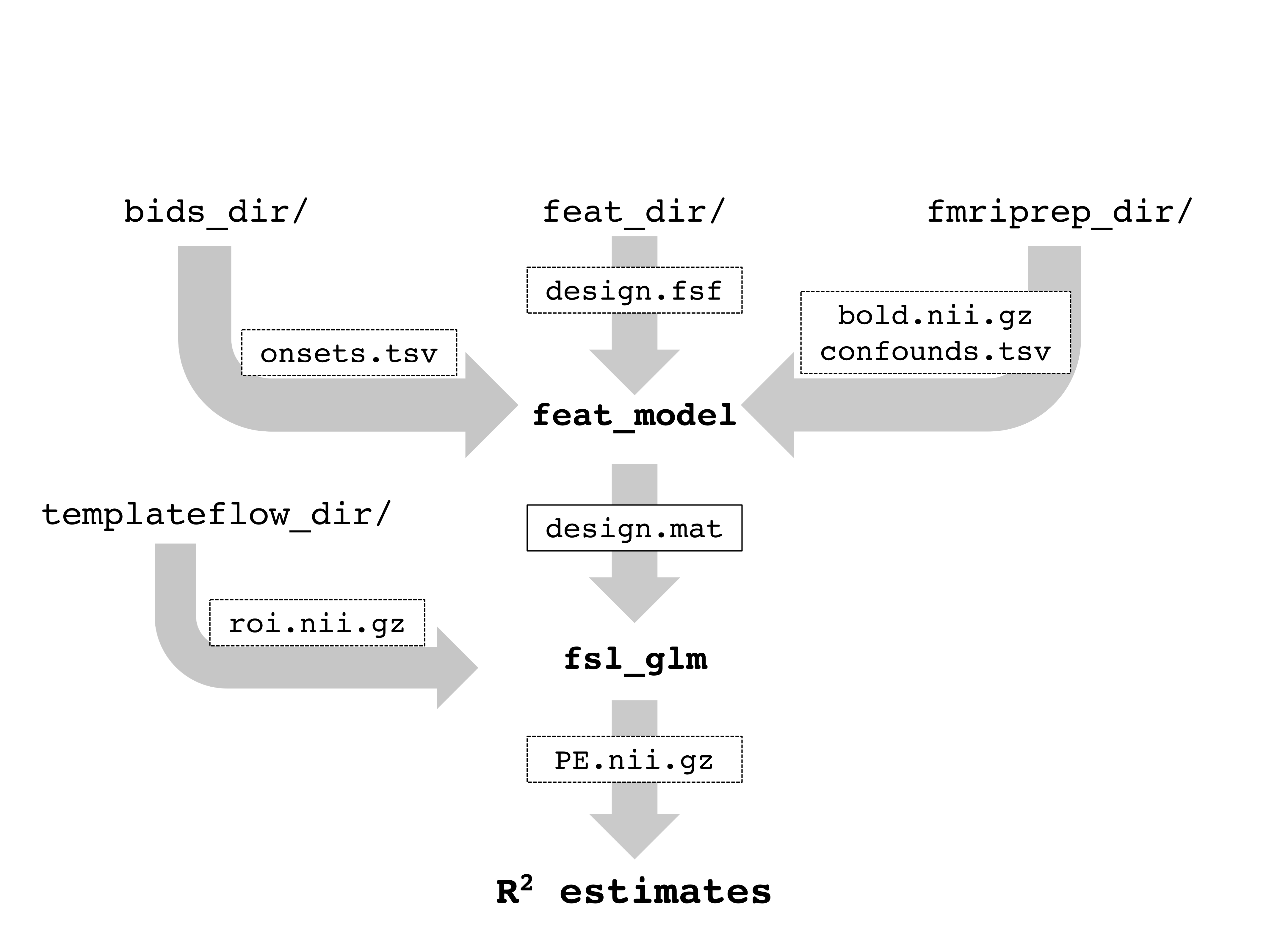
The confounder BIDS app is built on python 3.7, making use of nilearn^6-7, TemplateFlow⁸, and FSL⁹ functionality. The confounder app is designed to calculate regional R² goodness-of-fit for first-level, task-based GLM models including a series of neurobiologically reasonable combinations of confounds. The combinations of confounds are built using the philosophy of including both measure a of head motion and a measure derived from the anatomical signals, such as CSF and WM. Users supply the location of a valid BIDS directory, an associated fMRIPrep output directory with task-based BOLD scans normalized into MNI152NLin2009cAsym space, and a directory including an example FSL 1st-level design.fsf file using the custom 3-column format for jittered, event-related designs and the users’ choice of HRF function. Users can also specify a region to calculate the model fit over from the Harvard-Oxford cortical atlas, with the default being bilateral intracalcarine cortex. The basic workflow of the app (Fig. 1) is to extract the specified region from the TemplateFlow MNI152NLin2009cAsym Harvard-Oxford cortical atlas and coregister it to the preprocessed functional dataset. The user-supplied example design.fsf file is used as a template to create a new design.fsf file for a given subject and task run. FSL’s feat_model is used to create the design matrix file, and fsl_glm is used to calculate the parameter estimates, masked with the region-of-interest. R² values are calculated across the task-related parameter estimates for all runs. Twelve separate sets of confounds, extracted from the fMRIPrep-calculated confounds.tsv file, are tested iteratively including the six motion parameters, DVARS, and framewise displacement as the measures of head movement and the first anatomy CompCor component, first temporal CompCor component, and both the CSF and WM signals as measures of anatomical signal. The app outputs a JSON file with the R² values, as well as a series of plots showing the BOLD signal, the confounds, and the correlation between the BOLD signal and confounds.

Results

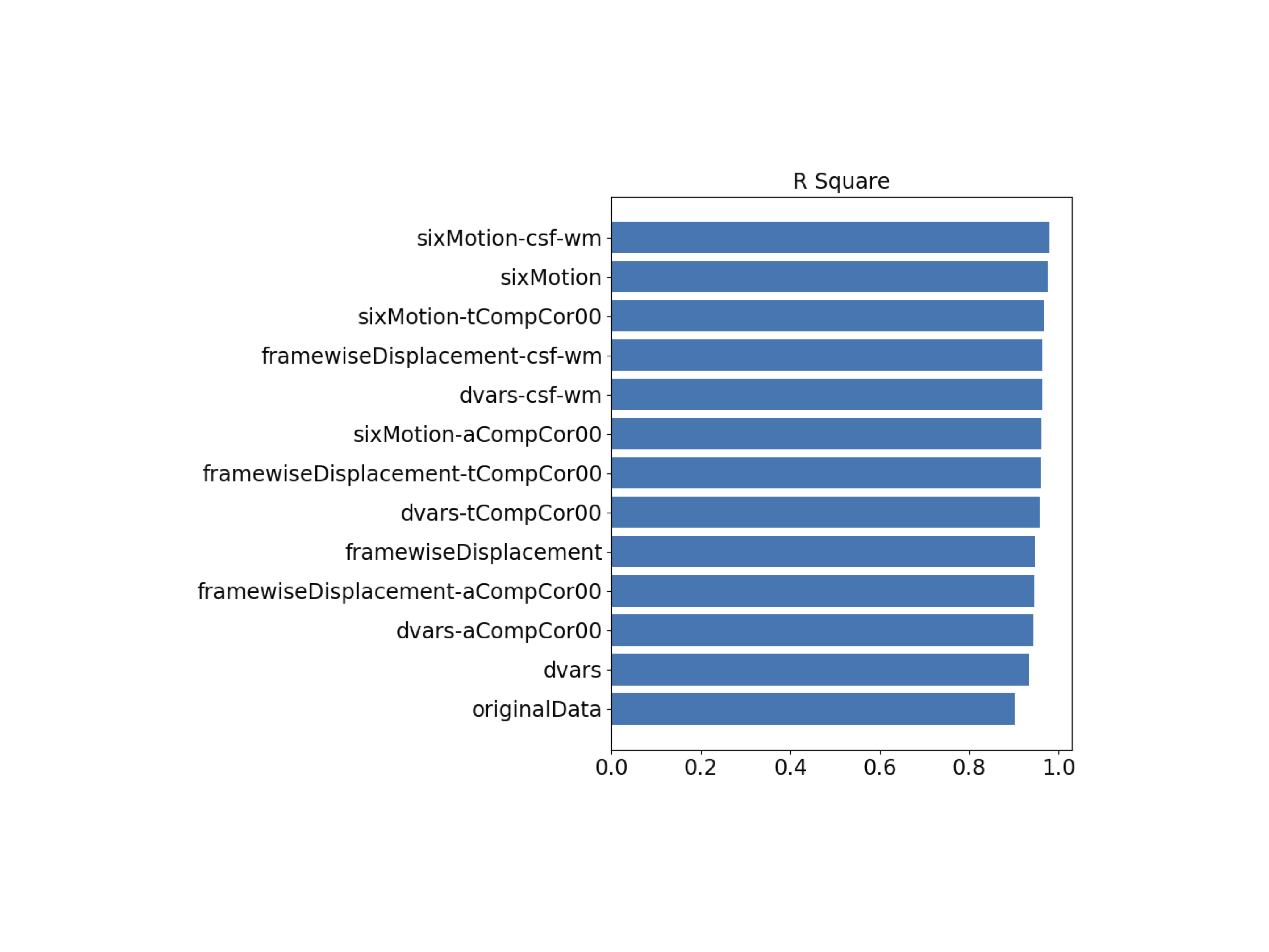
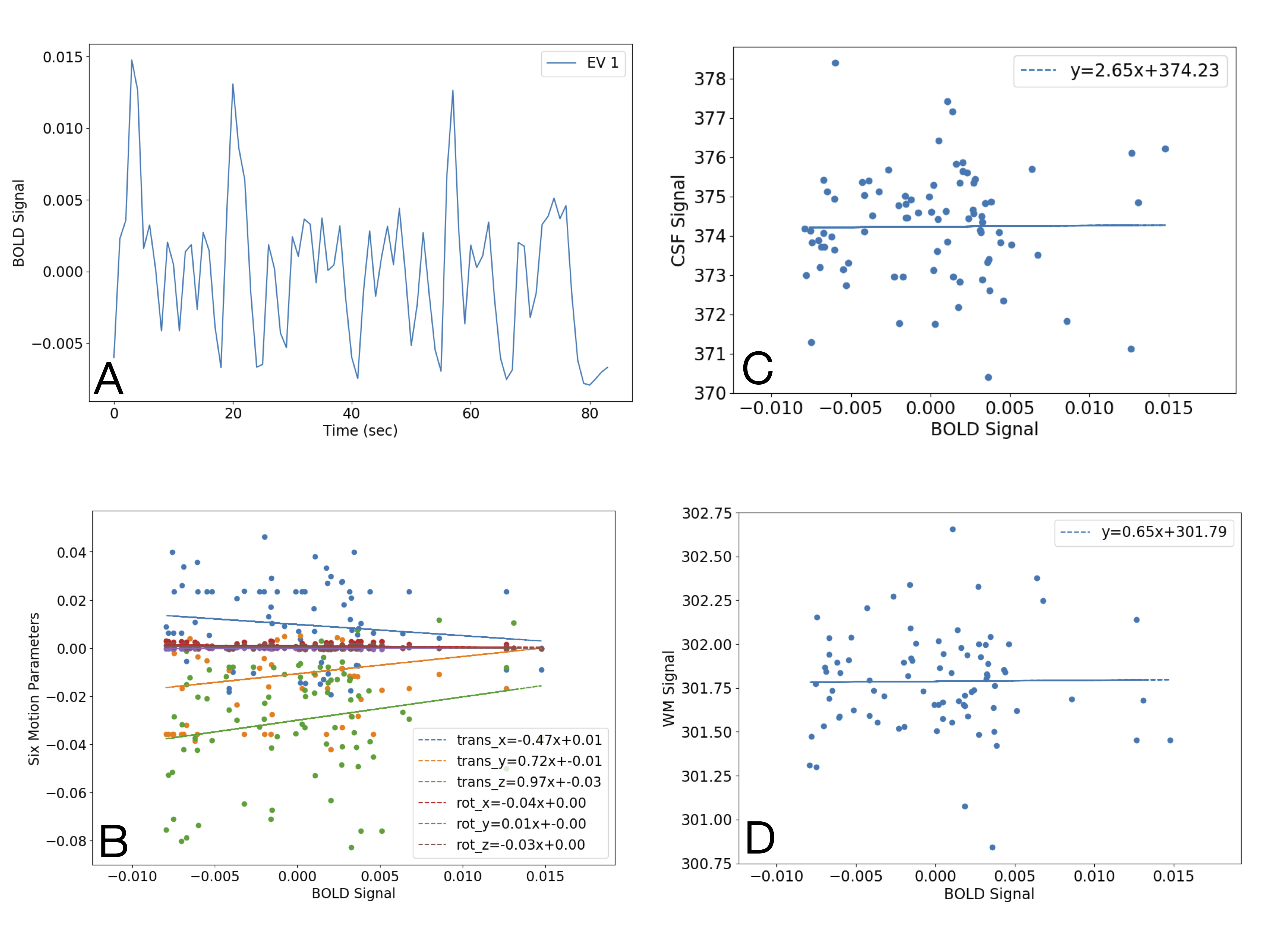
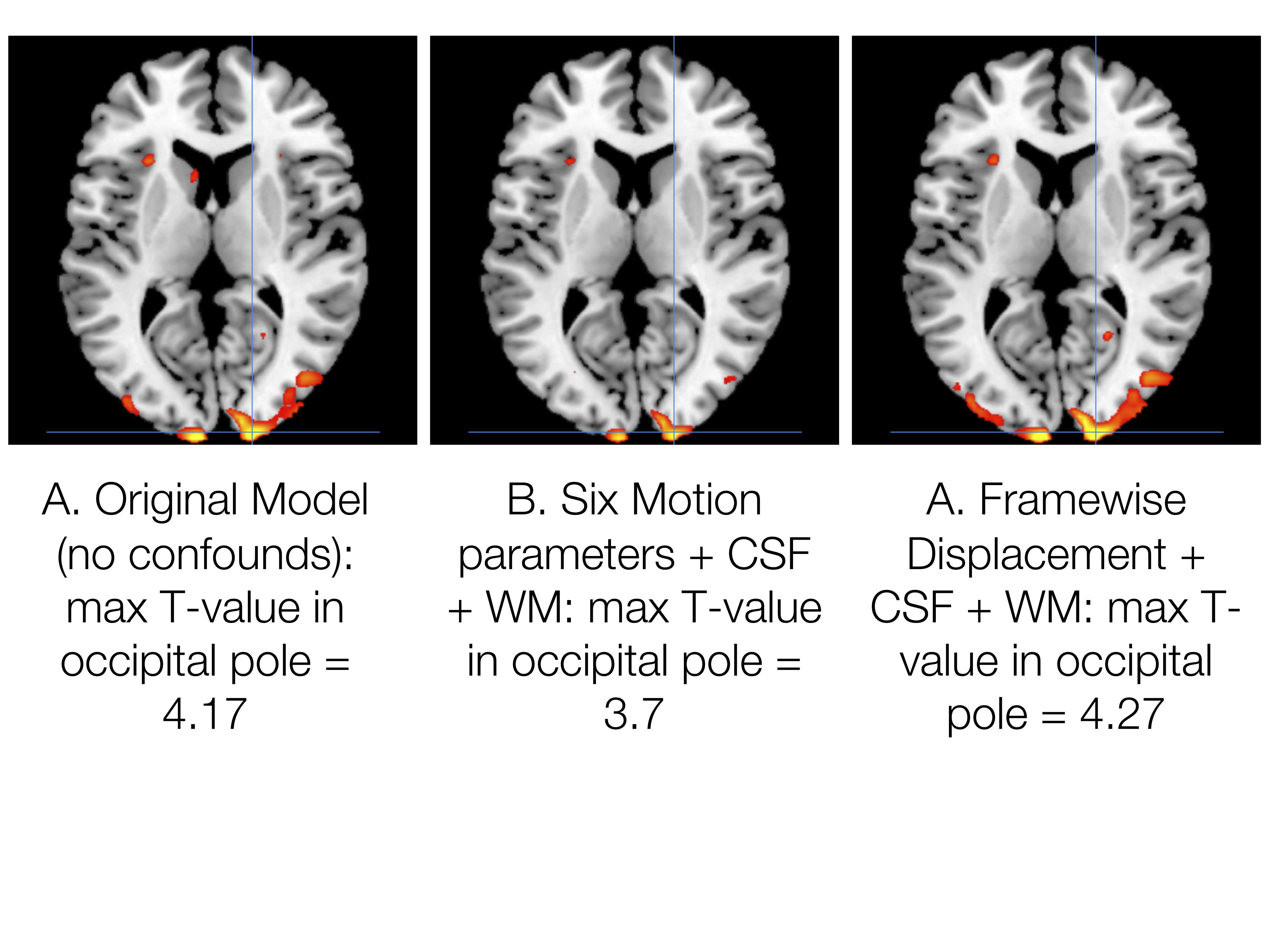
Using a single, healthy control subject performing five runs of a simple, decision-making task, the confounder app shows that the addition of any of the combinations of experimental confounds to the 1st-level GLM improves the R² fit of the model compared with the original model with only task regressors (Fig. 2). Fig. 3 shows exemplar output plots for the first run of the BOLD signal for the EV (Fig. 3A), along with plots showing the correlation between the EV and the confounds included in the model with the highest R² (Fig. 3B-D). When selecting confounds to include in a GLM, there will always be a trade-off between model fit and degrees of freedom, as can be seen from the peak T-statistic in a cluster in the right occipital pole (Fig. 4) estimated for the model including no confounds (T = 4.17), the model with the highest R² and most confounds (Six Motion+CSF+WM; T = 3.7), and the model with highest R² and fewest confounds (Framewise Displacement+CSF+WM; T = 4.27). In this case, the model with the highest R² but most confounds is not necessarily the best choice; rather a model with a slightly lower R² but fewer confounds appears to be a more optimal choice.

Conclusions

Here we present a new BIDS/fMRIPrep app, confounder, that allows users to efficiently assess model fit for first-level, task-based GLM models with and without experimental confounds. While the confounder app is not designed to provide a single answer as to which set of experimental confounds is best to include as covariates of no interest in a GLM, it does provide users with information to help guide this decision, including regional R², as well as additional information regarding data quality (e.g., correlation between confounds and predicted BOLD signal). These functionalities will allow it to expand on other BIDS apps such as fMRIPrep⁴ and MRIQC¹⁰ in creating a better set of task-based fMRI tools for the open fMRI community.

Acknowledgements

No acknowledgement found.