INTRODUCTION:

While schizophrenia patients have shown altered connectivity in central executive networks (CEN) and default mode network (DMN)¹, how the network nonlinear dynamics may be different in patients remains unknown. Phase space embedding has been widely used to examine the dynamics in nonlinear system².To investigate the network dynamics under resting-state conditions in schizophrenia, we modeled the reconstructed phase-space trajectory with a multivariate autoregressive model (MVAR). The derived AR coefficients were further analyzed with a linear discriminant analysis (LDA) to distinguish patients from controls. With this method, we found significant group differences in the dynamics within both CEN and DMN and between their interaction.

Methods:

Datasets
The first dataset is from the UCLA Consortium for Neuropsychiatric Phenomics LA5c. We selected 50 schizophrenia (SZ) patients and 50 age-matched healthy control (HC) subjects³. The second dataset is from the Center for Biomedical Research Excellence (COBRE). We selected 64 SZ subjects and 64 age-matched HC subjects⁴. Standard prepossessing, including despiking, slice time correction, motion correction, normalization, and smoothing, was performed on the resting-state functional magnetic resonance imaging (rfMRI) data using FSL⁵. CEN and DMN were then identified using concatenated group independent component analysis (ICA) via FSL Melodic⁶. Individual time courses of both networks were extracted using dual regression analysis⁶.
Single network dynamics
We constructed the phase space of the normalized ICA percentile time course $$$x_n$$$ for each subject, n is the length of the time course. We formed the matrix $$$Y$$$ related to the phase portrait as shown in eq. (1).
$$Y=(\mathbf{x}_t,\mathbf{x}_{t+\tau},\cdots,\mathbf{x}_{t+(m-1)\tau}), \qquad\qquad\qquad(1)$$


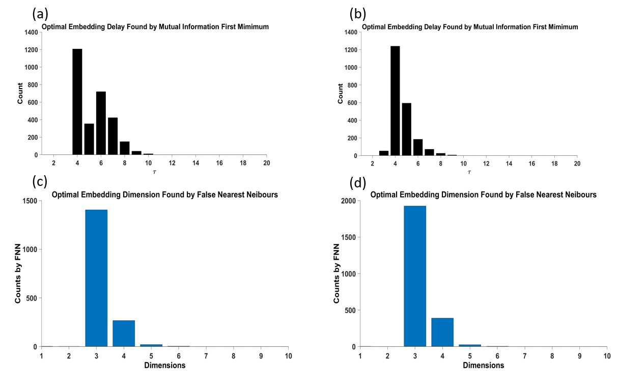
The optimal embedding dimension $$$m$$$ was determined by false nearest neighbor algorithm⁷ and the optimal embedding time delay $$$\tau$$$ was determined by minimization of the mutual information between the shifted time course.
After construction of the phase space, we used an MVAR model to compute the autoregression coefficients of the phase space⁸ as shown in eq. (2): $$ Y[j]=\sum_{i=1}^{P}a[j]Y[i-j]+\mathbf{e}[j],\qquad\qquad\qquad\quad (2)$$

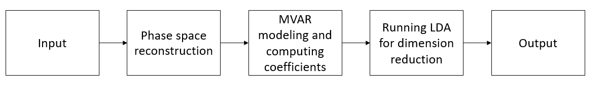
where $$$Y[j]$$$ is the $$$j^{th}$$$ row of $$$Y$$$, the model coefficients $$$A[i]$$$ are matrices of size $$$m×m$$$, $$$\mathbf{e}[j]$$$ is the error vector of the model, and $$$P$$$ is the order of the autoregression model. Thus, for each subject, we obtained $$$P×m×m$$$ coefficients. To reduce the number of features, a feature vector $$$\mathbf{x}$$$ corresponding to the largest eigenvalue was extracted with dimension $$$d_x$$$ less than $$$P×m×m$$$ using LDA. The autoregression order $$$P$$$ was set to 1. The entire approach is summarized in the flow diagram in Fig.1. The input is a normalized ICA percentile time course and the output is the feature vector $$$\mathbf{x}$$$.

Joint network dynamics of CEN and DMN
The joint phase space between the two networks, $$$Y_M$$$, was constructed as the following four-dimensional (we set $$$m$$$ equal to $$$1$$$ and $$$\tau$$$ equal to $$$4$$$) phase space matrix.
$$Y_M (t)=(\mathbf{c}_t,\mathbf{c}_{t+τ},\mathbf{d}_t,\mathbf{d}_{t+τ}), \qquad\qquad\qquad (3)$$
where $$$\mathbf{c}$$$ and $$$\mathbf{d}$$$ (length equals $$$n-(m-1)\tau$$$ ) represent the CEN and DMN percentile time series respectively. The model coefficients $$$A[i]$$$ had a size of size $$$4×4$$$ in this case. A similar process was performed to obtain the features.

RESULTS:

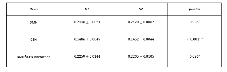
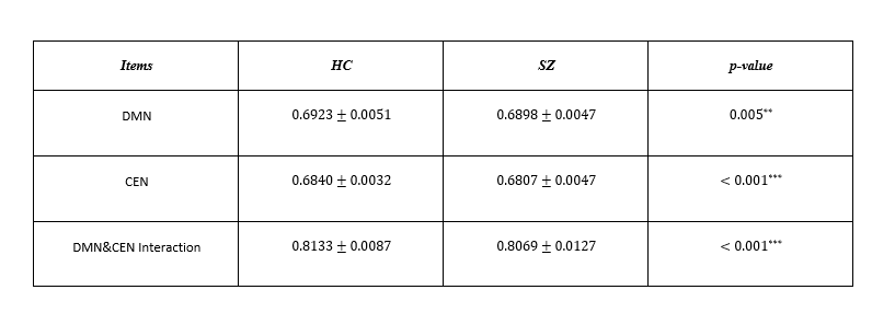
Model parameters, including the optimal dimension of embedding $$$m$$$ and the time delay $$$\tau$$$ for all the subjects are depicted in Fig.2. As shown in the histograms, for both UCLA and COBRE, the peak of the first minimum mutual information occurred at $$$\tau=4$$$. The peak of the optimal embedding dimension occurred at $$$m=3$$$. Therefore, we used these values in our experiments.

The comparison with the principal feature vector between SZ and HC for the two datasets is shown in Table I and II, respectively. ANOVA with post-hoc analysis using Fisher's Least Significant Difference (LSD) showed a significant difference between SZ and HC for both datasets ($$$p<0.05$$$) in CEN, DMN and their interaction.

DISCUSSION and CONCLUSION:

In this study, we investigated the dynamics of two key brain networks (CEN and DMN) and interactions between them using phase space embedding and autoregressive modeling. We found significant group differences in the principal feature of autoregression coefficients of phase space for both UCLA and COBRE datasets. The smaller autoregression coefficients values in schizophrenia may suggest greater stochasticity in the two networks. Our study indicates that phase space embedding along with autoregressive modeling may be useful to investigate the nonlinear dynamics of brain networks and their interaction in schizophrenia.

Acknowledgements

We acknowledge the use of the UCLA and COBRE datasets.