Introduction

Spatial smoothing is common when post-processing fMRI time-series. The impact on the temporal SNR (tSNR) depends on the baseline SNR, the intrinsic smoothness of the data (σ_I) and the characteristics of the physiological noise, including both amplitude (λ) and the degree of spatial correlation¹. Here we propose an extended model that additionally parameterises the degree of spatial correlation of the physiological noise (α). Furthermore, this model can be used to estimate σ_I, λ and α from just one time-series. We validate the model with simulated and in vivo 3T data. We replicate the finding that physiological noise increases with the number of segments with 3D-EPI².

Methods: Model extension

Consider a time series comprised of a mean signal $$$\bar{S}$$$ with variance components σ₀² and σ_p² arising from thermal and physiological noise processes respectively, with the physiological component varying with signal intensity³ (σ_p=λS).
Images have some intrinsic smoothness due to the acquisition and reconstruction processes. Applying an isotropic 3D Gaussian filter to a volume with spatially uncorrelated noise reduces the variance by $$$8\pi^{3/2}\sigma_F^3$$$ where σ_F is the standard deviation (SD) of the filter. Therefore, by approximating the intrinsic smoothness with such a filter, with SD=σ_I, the baseline SNR of the original images can be expressed as: $$$SNR_o=\frac{\bar{S}}{\sigma_0}\sqrt{8\pi^{3/2}\sigma_I^3}$$$.
Similarly, spatial smoothing with a filter with SD=σ_F decreases the noise variance without affecting the mean signal such that:$$$\left(\frac{SNR_{smooth}}{SNR_o}\right)^2=\frac{\sqrt{\sigma_I^2+\sigma_F^2}^3}{\sigma_I^3}=V\space\space(Eq.1)$$$. This ratio is denoted V for consistency with¹. We introduce an additional parameter α tuning the degree of spatial correlation in the physiological noise such that: $$$\sigma_{p_{smooth}}=\frac{\sigma_p}{1+\alpha\left(\sqrt{8\pi^{3/2}\sqrt{\sigma_I^2+\sigma_F^2}^3}-1\right)}$$$ . In the extrema, if α=0, the physiological noise is fully spatially correlated, such that smoothing does not reduce the variance, whereas if α=1, the physiological noise is spatially uncorrelated and smoothing reduces the variance in a manner equivalent to smoothing the thermal noise.
The tSNR of the smoothed time-series can therefore be expressed as:
$$tSNR_{smooth}=\frac{\bar{S}}{\sqrt{\sigma_{0_{smooth}}^2+\sigma_{p_{smooth}}^2}}=\frac{V.SNR_o}{\sqrt{V+V^2\lambda^2SNR_o^2\left(1+\alpha\left(\sqrt{V8\pi^{3/2}\sigma_I^3}-1\right)\right)^{-2}}}\space \space (Eq.2)$$

Methods: Validation

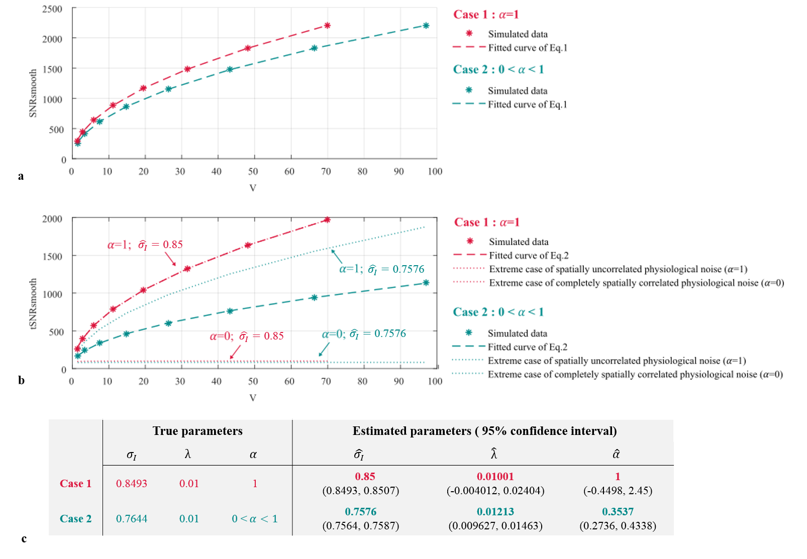
• Simulated data

A set of 50 volumes of dimension 30×30×30, was composed of a signal S, with additive random Gaussian noise, $$$\mathcal{N}(0,\sigma_0^2I_d)$$$ where I_d is the identity matrix. Each volume was smoothed with an isotropic 3D Gaussian filter (SD=σ_I ) to simulate the intrinsic smoothness of the data. The data were then smoothed with additional isotropic 3D Gaussian filters (SD=σ_F ) to simulate the effect of smoothing with variable kernels. SNR_o and SNR_smooth were computed as the ratio of the mean and SD across unsmoothed and smoothed volumes, respectively.
A second set of data were created as above, but with the additional factor of spatially correlated physiological noise, $$$\mathcal{N}(0,\sigma_p^2C)$$$ , added in the first step. tSNR_smooth was computed from these smoothed time-series. SNR_smooth,SNR_o and tSNR_smooth were then averaged across the centre portion of the grid (to avoid edge effects). The ratio $$$\left(\frac{SNR_{smooth}}{SNR_o}\right)^2 $$$ was fit to Eq.1 in order to estimate σ_I, which was subsequently used to fit tSNR_smooth to Eq. 2 to estimate α and λ.

Two cases were investigated. Physiological noise was either:
1./ Spatially uncorrelated: $$$C=I_d$$$
2./ Partially spatially correlated: C was a symmetric positive definite matrix with some off-diagonal elements non-null.

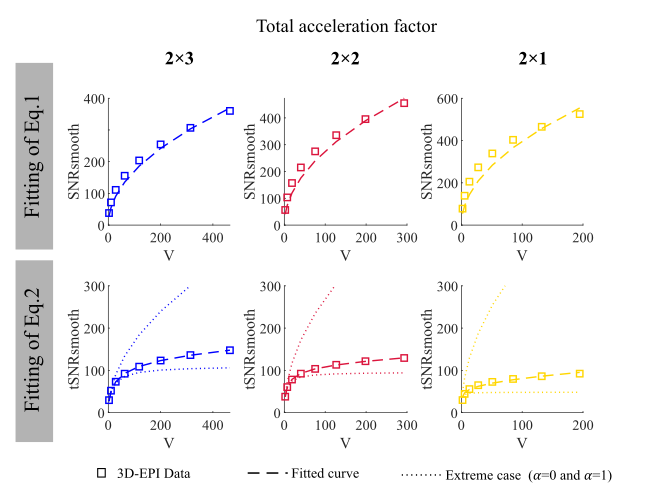
• In vivo data

Time-series of 100 volumes was acquired using an in-house⁴ 3D-EPI sequence on a 3T Siemens Prisma scanner and reconstructed with an in-house SENSE-based algorithm⁵. Key protocol parameters were: acquisition matrix 128x144x72, voxel size 1.5mm³, acceleration factors of 2 in-plane and 1, 2 or 3 through-plane, bandwidth 1776Hz/pixel, TR/TE 66/32.20ms.
SNR was computed using a Monte-Carlo method⁶. A set of replica volumes were reconstructed from the time-series’ mean k-space data with additive noise sampled from a distribution with the same statistics as the thermal noise obtained from the same protocols with no RF excitation. The replicas and the acquired volumes were smoothed with a 3D Gaussian filter with FWHM from 1 to 8 mm. SNR_o and SNR_smooth were computed as the ratio of the mean and the SD across replicas before and after smoothing, respectively. tSNR_smooth was computed in the same way from the acquired smoothed time-series after additional realignment and detrending. tSNR_smooth, SNR_o and SNR_smooth were averaged across grey matter (p(GM)>0.99) after correcting for non-Gaussianity⁷. The summary data were fit to (Eq.1) and (Eq.2).

Results

• Simulated data

The estimated $$$\hat{\lambda}$$$ and $$$\hat{\sigma_I}$$$ closely matched the true values in both simulated cases (Fig.1). In agreement with theory, $$$\hat{\alpha}$$$ was estimated to be 1 in the case of no spatial correlation and <1 in the other.

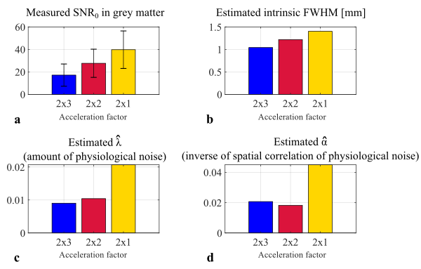
• In vivo data

The SNR of the different 3D-EPI protocols followed the expected trend of increasing as the acceleration factor decreased (Fig.3a). .
Fig.2 and Fig.3b-c-d show results of the model fitting. The estimated intrinsic smoothness followed the same pattern as the SNR. $$$\hat{\lambda}$$$ increased with the number of acquired partitions (from 0.009 to 0.0207), consistent with previous findings². $$$\hat{\alpha}$$$ was neither 0 nor 1 indicative of partially correlated physiological noise, as previously observed in¹.

Discussion

The extended model proposed here allows the full impact of smoothing to be characterised without the need to acquire several time series with variable baseline SNR to estimate the amplitude of the physiological noise(λ). The model results, validated via simulation and in vivo experiment, are consistent with literature.

Acknowledgements

The WCHN is supported by core funding from the Wellcome [203147/Z/16/Z].