3820
Temporal SNR in multiecho fMRI and its dependence on the choice of weights1Center for Functional MRI, UC San Diego, La Jolla, CA, United States, 2Biomedical Engineering, University of Southern California, Los Angeles, CA, United States, 3GE Healthcare, Buc, France, 4GE Healthcare, Waukesha, WI, United States, 5GE Healthcare, Menlo Park, CA, United States
Synopsis
In multi-echo fMRI, data from multiple echoes are combined using weights. We use the framework of the generalized Rayleigh quotient (GRQ) to derive the optimal weights for temporal SNR (tSNR) and multi-echo tSNR (metSNR) measures of performance. We also examine the sensitivity of both these measures to the choice of weights. We find that metSNR measures are relatively insensitive to the weights in gray matter regions as compared to tSNR measures, which show greater sensitivity in these regions. We interpret the findings using the form of the GRQ.
Introduction
A key step in multi-echo fMRI is the optimal combination of the data from multiple echoes. Posse et al [1] demonstrated that CNR was maximized with a matched filter weighting approach. However, subsequent studies reported that CNR was relatively independent of the choice of weights [2,3]. In this abstract, we consider two metrics of sensitivity that have been used to characterize the sensitivity of multi-echo fMRI: temporal SNR (tSNR) and multi-echo temporal SNR (metSNR) [2-4]. Using the framework of the generalized Rayleigh quotient, we derive optimal weights for both metrics and examine the relative sensitivity of the metrics to the choice of weights.Theory
We define $$$S$$$ as a $$$N_E \times N_T$$$ matrix where the $$$k$$$th row is the time series for the $$$k$$$th echo, $$$w$$$ as the $$$N_E \times 1$$$ vector of weights, and $$$\bar{S}$$$ as the $$$N_E \times 1$$$ vector consisting of the temporal means. With this notation we have$$\textrm{tSNR} = \frac{mean(w^T S)}{std(w^T S)} = \frac{w^T \bar{S}}{std(w^T S)}$$
To maximize the tSNR, we can consider maximizing its squared version
$$\left( \textrm{tSNR} \right) ^2 = \frac{w^T \bar{S} \bar{S}^T w}{var (w^T S)} = \frac{w^T A w}{ w^T \Sigma w}$$
where $$$A = \bar{S} \bar{S}^T$$$ and $$$ \Sigma = E \left[ \left(S - \bar{S} \right) \left( S- \bar{S} \right)^T \right] $$$ is the covariance matrix. The expression for $$$(tSNR)^2$$$ has the form of a generalized Rayleigh quotient which is maximized when the weight vector has the form $$$w = k \Sigma^{-1} \bar{S}$$$ where $$$k$$$ is an arbitrary scalar [5]. From the form of $$$(tSNR)^2$$$ it is straightforward to see that tSNR will be relatively invariant to the choice of weights when $$$A = \bar{S} \bar{S}^T \approx \Sigma$$$.
For a single echo acquisition, tSNR is proportional to CNR. For multi-echo acquisitions, a multi-echo variant of tSNR that is proportional to CNR is defined as [2,3]:
$$ \textrm{metSNR} = \frac{mean(w^T D_{\tau} S) }{std(w^T S)} = \frac{w^T D_{\tau} \bar{S}}{std(w^T S)}$$
where $$$D_{\tau} = diag ( [ TE_1, TE_2,...,TE_{N_E} ] )$$$. The optimal weight vector for metSNR has the form $$$w = k \Sigma^{-1} D_{\tau} \bar{S}$$$. When $$$\Sigma = I$$$, then $$$w = k D_{\tau} \bar{S}$$$ is equivalent to the matched filter solution originally proposed in [1], since the elements of $$$\bar{S}$$$ are proportional to $$$exp(-TE_i/T_2^*)$$$. metSNR will be relatively invariant to the choice of weights when $$$B = D_{\tau} \bar{S} \bar{S}^T D_{\tau}^T \approx \Sigma$$$.
Methods
Resting-state fMRI data (eyes-closed) were acquired from one healthy male on a GE MR750 3T system with a 32-channel receive head coil and a multi-echo multiband EPI sequence with the following parameters: TR = 1.3 s; θ = 52°; FOV = 192 mm; matrix size = 64×64; 48 3mm thick slices, multiband factor = 3; TE=[12.2 30.1 48.0] ms, 277 reps; scan time = 6 min. Data were preprocessed using the meica.py [4] script (v2.5b11) with 2nd order polynomial detrending, default despiking, and no smoothing.For each voxel we computed values of tSNR and metSNR with different choices for the weights. These included the optimal weights for tSNR and metSNR. We also considered 3 variations of the optimal tSNR weight vector: (1) $$$w_{swt} = \bar{S}$$$; (2) $$$w_{tdg} = \Lambda^{-1} \bar{S}$$$ where $$$\Lambda$$$ is the diagonal portion of $$$\Sigma$$$, and (3) $$$w_{tsnr} = \Lambda^{-0.5}\bar{S}$$$. In addition, we considered 4 variations of the optimal metSNR weight vector: (a) $$$w_{BS} = D_{\tau} \bar{S}$$$ , (b) $$$w_{t2wt} = D_{\tau} exp(-TE/T_2^*)$$$ where $$$TE$$$ is the vector of echo times, (c) $$$w_{mdg} = \Lambda^{-1} D_{\tau} \bar{S}$$$, and (d) $$$w_{mdg} = \Lambda^{-0.5} D_{\tau} \bar{S}$$$. Variations (a) and (b) are equivalent to the matched filter weights in [1], with minor differences due to estimation error of $$$T_2^*$$$. Variations (3), (a), and (d) are equivalent to the tSNR, BOLD sensitivity, and temporal BOLD sensitivity weightings in [3]. In addition, we also consider a uniform weighting of the form $$$w_{flat}= 1$$$.
Results and Conclusion
Fig. 1 shows tSNR and metSNR maps for the different weight variants, normalized using tSNR and metSNR values obtained using the respective optimal weights. For the metSNR-based weight variants, the normalized metSNR maps shows values in GM and WM regions that are close to the optimal value of 1.0.As noted in theory, tSNR and metSNR will be relatively robust to weight choice when $$$\Sigma$$$ is similar to A and B, respectively. Fig. 2 shows that the cosine similarity between $$$\Sigma$$$ and A is larger in CSF regions whereas the similarity between $$$\Sigma$$$ and B is larger in GM regions. Plots of these quantities for representative GM, CSF, and WM voxels are also shown.
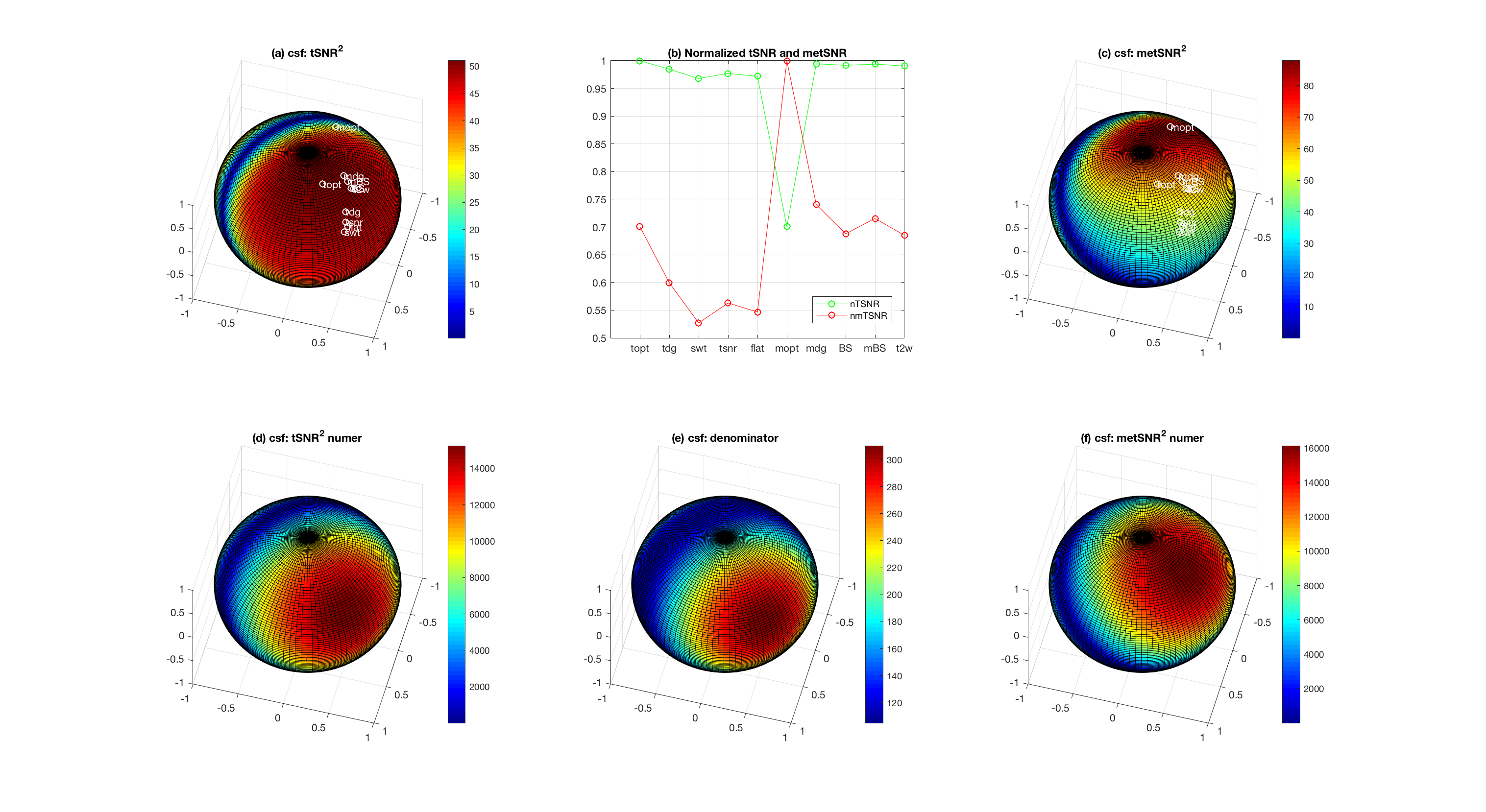
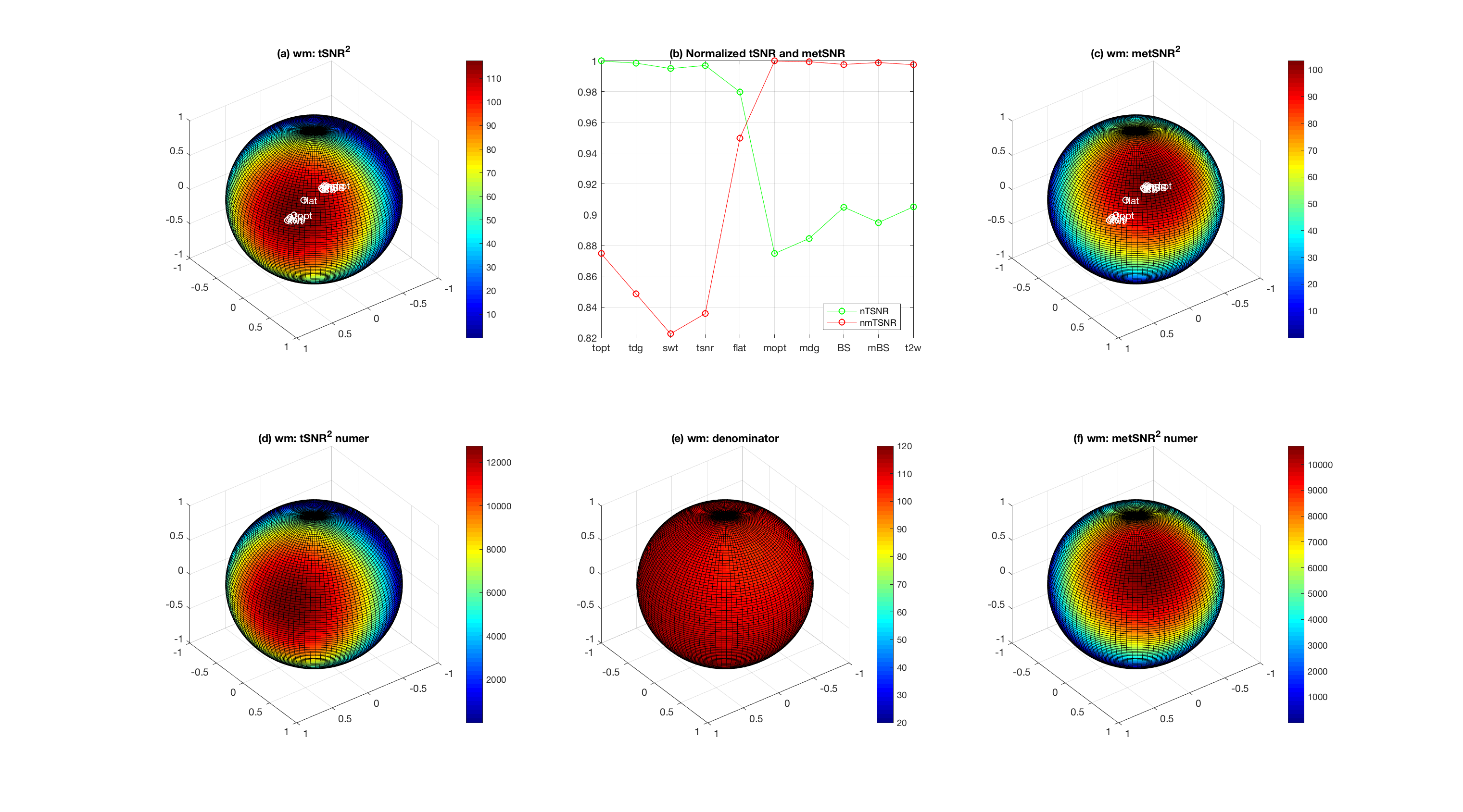
The spherical plots in Figs 3-5 show how the weight sensitivities of $$$metSNR^2$$$ and $$$tSNR^2$$$ depend on the similarity of the numerator and denominator terms, with $$$metSNR^2$$$ being less sensitive for the GM voxel due to the similarity between $$$w^T B w $$$ and $$$w^T \Sigma w $$$ and $$$tSNR^2$$$ less sensitive for the CSF voxel due to similarity between $$$w^T A w $$$ and $$$w^T \Sigma w $$$.
As noted in [2,3], metSNR is proportional to CNR for multi-echo fMRI and is thus the preferred metric for evaluating in-vivo performance. For GM regions, metSNR is relatively robust to the weight choice due to the similarity of B and $$$\Sigma$$$.
Acknowledgements
This project was supported in part by in-kind support from GE Healthcare.References
[1] Posse, S., Wiese, S., Gembris, D., Mathiak, K., Kessler, C., Grosse-Ruyken, M. L., Elghahwagi, B., Richards, T., Dager, S. R., Kiselev, V. G., Jul. 1999. Enhancement of BOLD-contrast sensitivity by single-shot multi-echo functional MR imaging. Magnetic resonance in medicine : official journal of the Society of Magnetic Resonance in Medicine / Society of Magnetic Resonance in Medicine 42 (1), 87–97.
[2] Poser, B. A., Versluis, M. J., Hoogduin, J. M., Norris, D. G., Jun. 2006. BOLD contrast sensitivity enhancement and artifact reduction with multiecho EPI: parallel-acquired inhomogeneity-desensitized fMRI. Magnetic resonance in medicine : official journal of the Society of Magnetic Resonance in Medicine / Society of Magnetic Resonance in Medicine 55 (6), 1227–1235.
[3] Kettinger, Á., Hill, C., Vidnyanszky, Z., Windischberger, C., Nagy, Z., 2016. Investigating the Group- Level Impact of Advanced Dual-Echo fMRI Combinations. Frontiers in neuroscience 10, 571.
[4] Kundu, P., Brenowitz, N. D., Voon, V., Worbe, Y., Vertes, P. E., Inati, S. J., Saad, Z. S., Bandettini, P. A., Bullmore, E. T., Oct. 2013. Integrated strategy for improving functional connectivity mapping using multiecho fMRI. Proceedings of the National Academy of Sciences of the United States of America 110 (40), 16187–16192.
[5] Monzingo, R., Haupt, R., Miller, T., 2011. Introduction to Adaptive Arrays, 2nd Edition. Scitech Publishing, Raleigh, NC.
Figures
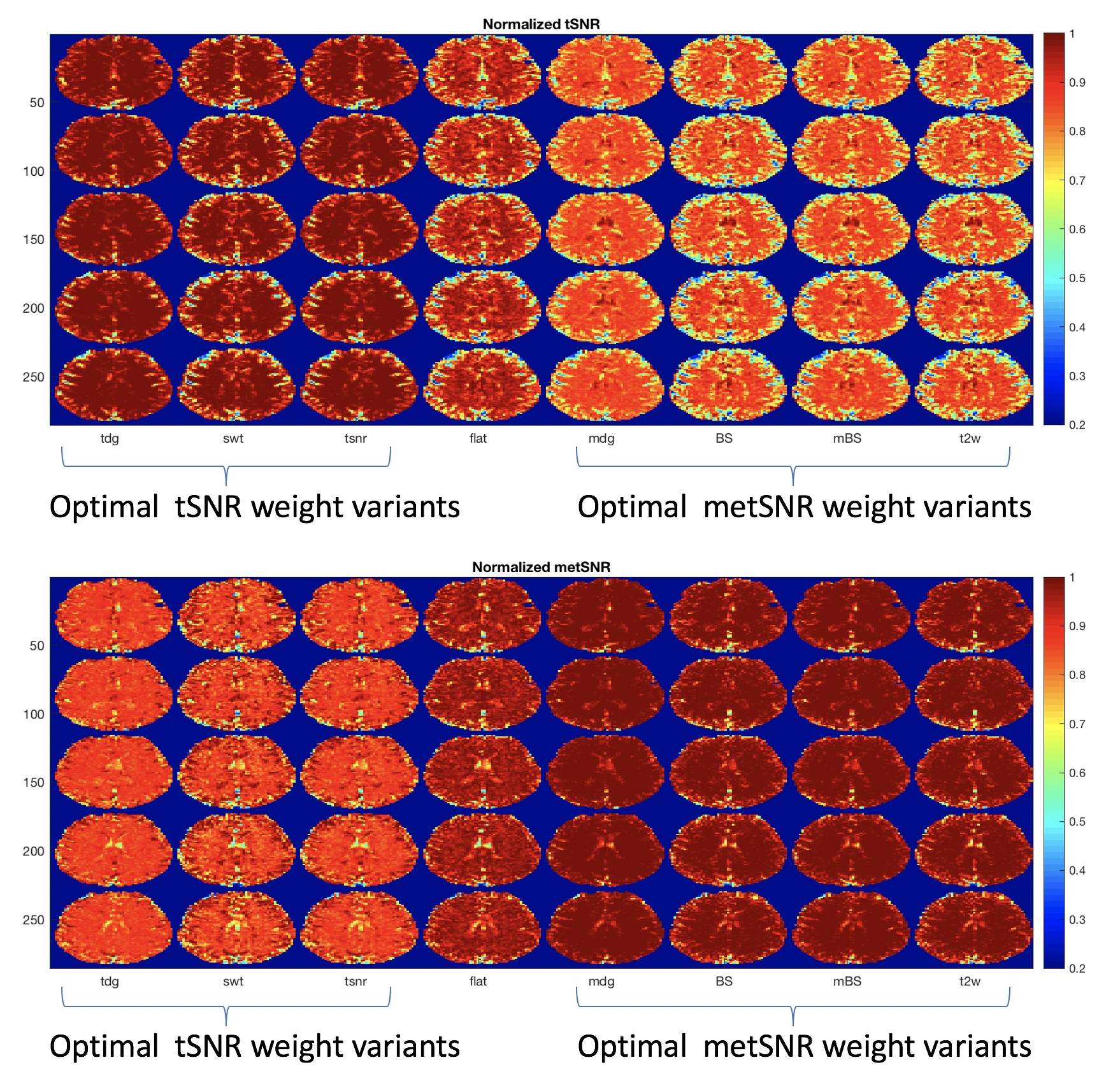
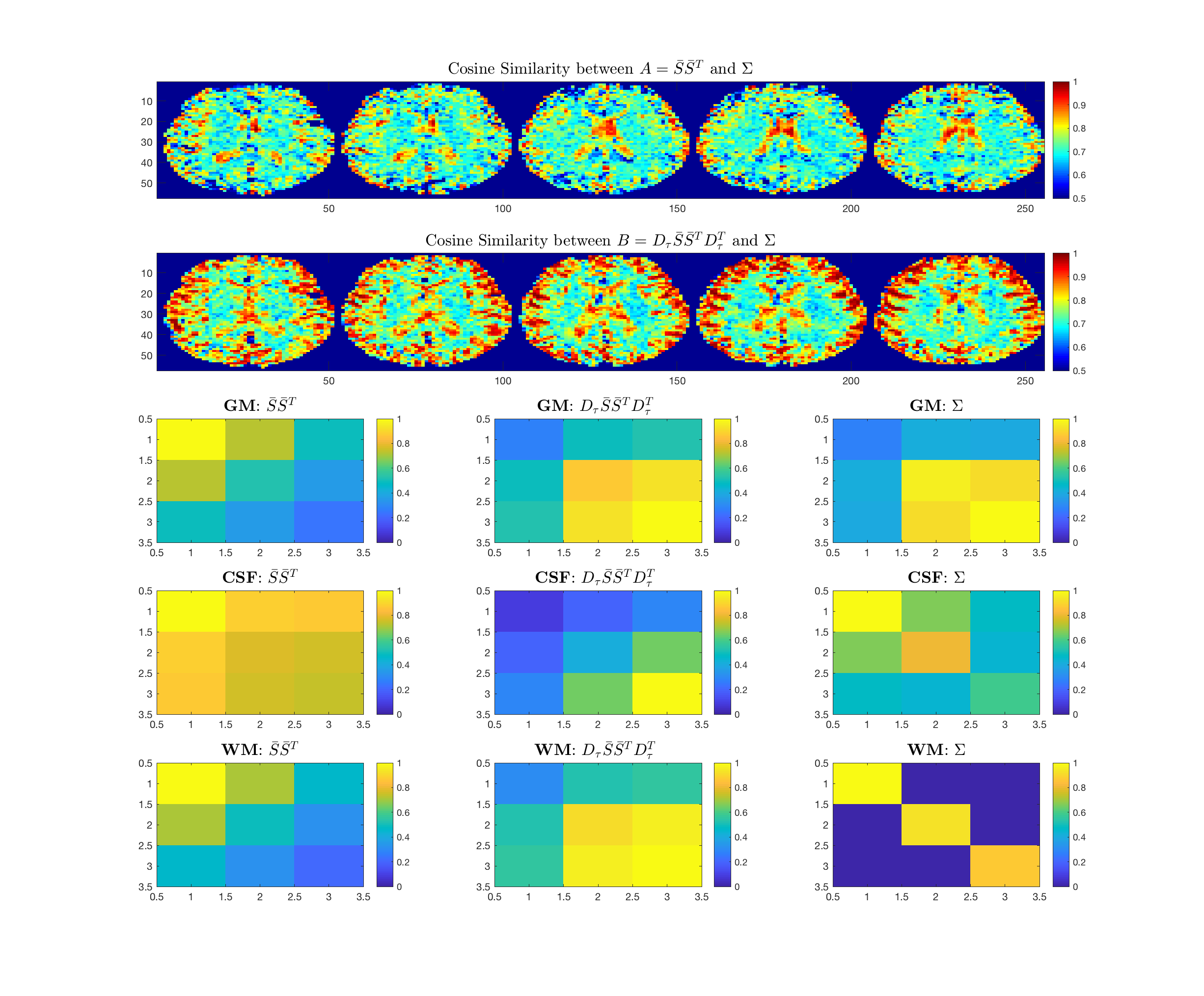
Fig 2. Row 1: Cosine similarity between A and C=$$$\Sigma$$$. Voxels with greater similarity will show greater invariance of tSNR to choice of weights. Row 2: Cosine similarity between B and C . Voxels with greater similarity will show greater invariance of metSNR to weight choice. Rows 3-5: Plots of A, B, and C for representative GM, CSF, and WM voxels. For GM voxel, B is more similar to C, so metSNR will show greater invariance to weight choice. For CSF voxel, A is more similar to C, so tSNR will show greater invariance.
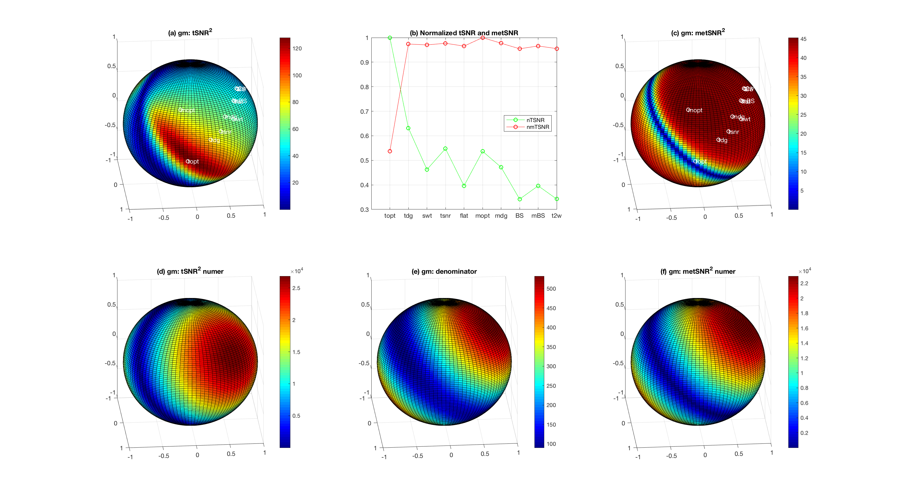
Fig 3. (a,c): tSNR^2 and metSNR^2 values as a function of weights, displayed on a 3D spherical surface for the GM voxel from Fig. 2. Panel b: tSNR and metSNR values for different weight variants. Both metrics have relatively low values when the optimal weight vector for the other metric is used. Panels (d): $$$X = w^T A w$$$; (e): $$$Z=w^T \Sigma w$$$; (f) $$$Y=w^T B w$$$. Note that tSNR^2 = X/Z and metSNR^2 = Y/Z. All quantities displayed as a function of weight on spherical surface. Because of greater similarity between Y and Z, the metSNR^2 sphere shows greater invariance to weight choice.