INTRODUCTION

The use of Transcranial Direct Current Stimulation (tDCS) is largely used for treatment of neurologic and psychiatric disorders$$$^{1,2}$$$. However, to clarify the underlying mechanisms, the spatial distributions of the electric current inside the brain, as well as the neural activation during the exam, is necessary. Along the years, there were a lot of efforts to map these distributions, mainly with simulated data$$$^{3}$$$. Recently, one group proposed the use of Magnetic Resonance Imaging (MRI) to map the tDCS induced magnetic field ($$$tDCS-\triangle B_{z}$$$), however, for head experiments only group level analysis was employed instead of individual mapping$$$^{4}$$$. According to the Ampere’s Law, electric currents generate magnetic fields. MRI is a powerful imaging modality which enables the detection of magnetic field changes along the main magnetic field axis (z-axis), reflected on the form of phase changes.

$$\triangle \phi_{(\overrightarrow{r}')}=-\gamma\triangle B_{z(\overrightarrow{r}')}TE$$

Since $$$\triangle B_{z(\overrightarrow{r}')}$$$ is reflected by changes in phase, it is necessary a careful processing of phase images, these include phase unwrapping, coregistration, realignment. This is necessary since any error on any preprocessing step may be confounded as a detected signal.
Another problem is that the order of magnitude of these induced magnetic fields are of nT, which requires a high Signal-to-Noise Ratio (SNR) to distinguish noise from magnetic field changes.
On this work, two different $$$tDCS-\triangle B_{z}$$$ mapping methodologies were tested, considering different mathematical approaches.

METHODS

For the tDCS experiment setup, a HD configuration was implemented with the anode at FC3 and the four cathodes at F3, FC1, FC5 and C3.
MRI images were acquired in a 3T scanner using a Gradient Echo sequence (two echos, TE = 2.3/4.6 ms, TR = 370 ms, voxel size 3x3x4 mm and flip angle 80°). The subjects showed no evidence of neurologic or neuropsychiatric disorders.
A dynamic acquisition was made with four blocks of Rest (8 scans each) interleaved with 3 blocks of Stimulus (10 scans each). For the Stimulus, in each block, a different current intensity was used (1, 2 and 3 mA for Subject 1; and 1, 1.5 and 2 mA for Subject 2). Between blocks there was one scan for Ramps (up and down). For each subject, the procedure was repeated once.
Phase images were preprocessed using SPM. All the parameters were calculated using the Magnitude images (first echo) and then applied to the phase images. The phase difference was calculated. For the $$$tDCS-\triangle B_{z}$$$ mapping, two different approaches were used.

Method 1: For each block, the mean along scans were calculated, resulting on four Rest volumes and three Stimulus volumes (Stim1, Stim2 and Stim3). With the four Rest volumes, the mean was calculated (Rest). Then, the magnetic field was estimated as follows:
$$B_{z}=\frac{[(\frac{Stim1}{J_{1}}-Rest)+(\frac{Stim2}{J_{2}}-Rest)+(\frac{Stim3}{J_{3}}-Rest)]}{3}$$
The idea was that the only difference between each block was the induced magnetic field, therefore, the Rest condition contained phase information to exclude from the Stimulus conditions. Also, since there is a linear relationship between magnetic field and electric current, a normalization was made for the electric current.As a final step, a background filter Projection onto Dipole Fields was used to eliminate the magnetic fields distributions induced by susceptibility sources inside the brain.

Method 2: A GLM was applied to the dynamic acquisition, with the electric current modeled as:
$$\overrightarrow{J}=\overrightarrow{J}_{off}+\overrightarrow{J}_{tDCS}+\overrightarrow{J}_{motion}$$
Where the $$$\overrightarrow{J}_{off}$$$ was modeled on GLM as an offset parameter, and the motion was modeled as a regressor associated to the movement along the scans. For each Stimulus block, a task block was given according to the intensity of the applied electric current, with this all the signal that do not variate linearly with the current is rejected.

Simulation: For a comparison, a simulated magnetic field distribution was also calculated using a simulated electric current distribution with Finite Element Model. With the vector of the electric current (three volumes, one for each axis of the 3D space), the magnetic field distribution was calculated according to the Biot-Savart Law, as a 3D Convolution of the current distribution $$$\overrightarrow{J}_{(\overrightarrow{r}')}$$$ and the function $$$\overrightarrow{h}_{(\overrightarrow{r}')}$$$.
$$\overrightarrow{B}_{(\overrightarrow{r})}=\frac{\mu_{0}}{4\pi}\int_{V'}^{}\overrightarrow{J}_{(\overrightarrow{r}')}\times\overrightarrow{h}_{(\overrightarrow{r}')}d^{3}r'$$
$$\overrightarrow{h}_{(\overrightarrow{r}')}=\frac{(\overrightarrow{r}-\overrightarrow{r}')}{|\overrightarrow{r}-\overrightarrow{r}'|^{3}}$$

RESULTS AND DISCUSSION

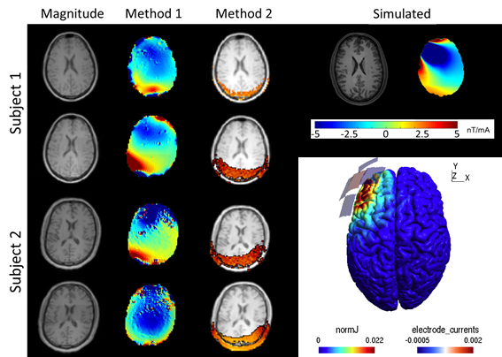
Figure 1 shows the estimated $$$tDCS-\triangle B_{z}$$$ mappings for the two subjects (both methods), at an axial slice. The simulated data is also presented, as well as the magnitude images at the same slice.
The first method showed some similarities with the simulated data, except for one case (Subject 2, second map), possibly due to the influence of noise and movement artifacts. As for the second method, there were only signal at the occipital region, while there were also expected signal at the frontal right side. A study concerning imaging parameters (such as TE, voxel size, etc) in order to improve the SNR is still necessary.As a preliminary study, the results points towards the possibility of mapping the magnetic field distributions induced by electric currents.

CONCLUSION

Of the tested methodologies, the first seemed to give better results than the second, possibly because the GLM method uses statistical approaches, thus, at low SNR the statistical testing won’t work. This suggests that the magnetic field mapping induced by HD-tDCS’s electric currents may be possible. However, a careful study about both methodologies and imaging parameters is still necessary.

Acknowledgements

As a part of Cognitive Rehabilitation Platform (CRP) Project, this research was funding and supported (with Grant number 2013/07375-0) by The Center for Research, Innovation and Diffusion of Mathematical Sciences Center Applied to Industry (CEPID-CeMEAI) of Sao Paulo Research Foundation (FAPESP), based at the Institute of Mathematics and Computer Sciences (ICMC) USP São Carlos.