Introduction

Magnetic resonance (MR) relaxometry yields the distribution of $$$T_2$$$ values within a sample or voxel, and can identify water compartments within tissue^1,2. For a two-compartment system, signal intensity at time $$$nTE$$$ is: $$s(nTE)=c_A\ e^{-nTE/T_{2,A}}+c_B\ e^{-nTE/T_{2,B}}\hspace{12pt}[1]$$where $$$c_i$$$ and $$$T_{2,i}$$$ denote size and relaxation time of compartment $$$i$$$, and $$$TE$$$ is the echo spacing. Estimation of $$$c_i$$$ and $$$T_{2,i}$$$ from multiexponential (ME) decay data is a classically ill-posed inverse problem, related to the inverse Laplace transform, with highly noise-dependent solutions. Relaxometry may be extended to 2D through incorporation of an additional variable. For $$$T_1-T_2$$$ experiments using inversion-recovery with inversion-time $$$TI$$$, signal intensity is:³$$s(TI,nTE)=c_A(1-2e^{-{TI}/T_{1,A}})e^{-{nTE}/T_{2,A}}+c_B(1-2e^{-{TI}/T_{1,B}})e^{-{nTE}/T_{2,B\ \ }}\hspace{12pt}[2]$$This generalizes to other 2D experiments, e.g. $$$T_2-D$$$, and to 3D experiments, e.g. $$$T_1-T_2-D$$$ incorporating diffusion through variable $$$b$$$ value⁴. We have shown empirically that the stability of parameter estimates from 2D experiments is superior to that from 1D experiments⁵ ; here, we provide statistical theory to demonstrate this, and present additional Monte Carlo simulations and experimental results in support of this theory.

Methods

We analyze the variances of parameters obtained from non-linear least squares (NLLS) fitting and its 2D extension.

Linear theory: The linear least-squares problem:$${\bf a^\ast}=\underset{a}{\operatorname{argmin}} ‖{\bf Ga-y}‖_2^2\hspace{12pt}[3]$$has the formal solution:$${\bf {a}^\ast}=({\bf G^TG})^{-1}{\bf G^{T}y}\hspace{12pt}[4]$$where $$$\bf y$$$ is the observed data vector, $$$\bf G$$$ is the design matrix defined by the specific experiment undertaken, and $$$\bf a$$$ is the vector of unknown parameters. For uncorrelated data with constant variance $$$\sigma^2$$$, one has $$$\operatorname{cov}({\bf {a}^\ast})=({\bf G^TG})^{-1}\sigma^2$$$, with the diagonal elements of $$$\operatorname{cov}({\bf {a}^\ast})$$$ representing the variances of the estimated parameters.

Linearized nonlinear theory: For the nonlinear case⁶,$${\bf a^\ast}=\underset{a}{\operatorname{argmin}}‖{\bf G(a)-y}‖_2^2\hspace{12pt}[5]$$ where $$$\bf G$$$ is a vector-valued function. The expansion of the i-th element of $$${\bf G}({\bf a})$$$ about $$$\bf a_0$$$, close to $$$\bf a^\ast$$$, is:$$G_i({\bf a_0+h})≈G_i({\bf a_0})+∑_k\frac{\partial G_i}{\partial a_k}|_{\bf{a_0}}h_k$$where $$$\bf h$$$ is a small increment vector with $$$\bf a=a_0 + h$$$, and fit parameters are indexed by $$$k$$$. Denoting the Jacobian of $$$\bf G$$$ at $$$\bf a_0$$$ as $$$B_{ik}=\frac{\partial G_i}{\partial a_k}|_{\bf{a_0}}$$$, Eq.[5] becomes:$${\bf a^\ast}\approx\underset{a}{\operatorname{argmin}} ‖{\bf Ba}+({\bf G}({\bf a_0})-{\bf Ba_0}-{\bf y})‖_2^2\hspace{12pt}[6]$$Eq.[6] is of the form of Eq.[3], so

$$\operatorname{cov}({\bf{a}^\ast})=({\bf B^TB})^{-1}{\bf B^T}\operatorname{cov}({\bf G}({\bf a_0})-{\bf Ba_0}-{\bf y})(({\bf B^TB})^{-1}{\bf B^T})^{\bf T}$$ Since $$${\bf G}({\bf a_0})$$$ and $$$\bf Ba_0$$$ are constants, $$\operatorname{cov}({\bf G}({\bf a_0})-{\bf Ba_0}-{\bf y})=\operatorname{cov}({\bf y})={\bf Id}\sigma^2$$ where $$$\bf Id$$$ is the identity; thus:$$\operatorname{cov}({\bf a^\ast})=({\bf B^TB})^{-1}\sigma^2\hspace{12pt}[7]$$

Linearized nonlinear 2D problems: For $$$T_1-T_2$$$ relaxometry (Eq.[2]), the two independent measurement times are defined by the grid $$$\rho_{k,n}=\{TI_k,nTE\}$$$, with data represented as a matrix³. Spin-echo data are obtained for a sequence of TI’s. The minimization objective function is a double sum over the 2D array of measurement points, with the ordering of points immaterial. For Eq.[2] the model space is $$$\textbf{a}=\{c_A,c_B,T_{1,A},T_{1,B},T_{2,A},T_{2,B}\}$$$. The 6 columns of $$$\bf B$$$ can be written as the vectorization of $$$\bf ρ$$$, with corresponding vectorization of the data matrix. The calculation of $$$\operatorname{cov}(\textbf{a})$$$ then follows as for the 1D case. We can now evaluate the accuracy of parameter estimates for particular 2D models.

Experimental methods: As a surrogate for noise realizations, gel experiments were performed with parameter estimates separately derived from each pixel, since underlying parameter values are relatively constant, but each voxel is contaminated by different noise. 1D T₂ and 2D T₁-T₂ experiments were performed on a 30% peanut oil/agar gel phantom at 300K using a Bruker 9.4T Avance III microimaging spectrometer. A multi-echo SE sequence with TE=8ms was used to generate 64 T₂-weighted images. For 2D experiments, this was preceded by inversion and a variable delay TI, repeated for 24 values of TI from 10μs to 10s. Pixel intensities were fit by NLLS, yielding $$$c_A,c_B,T_{1,A},T_{1,B},T_{2,A}$$$ and $$$T_{2,B}$$$ for each of 1881 pixels.

Results

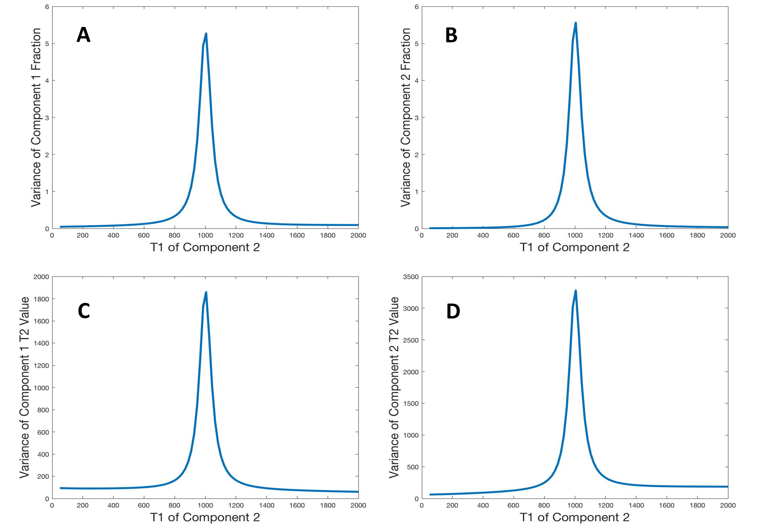
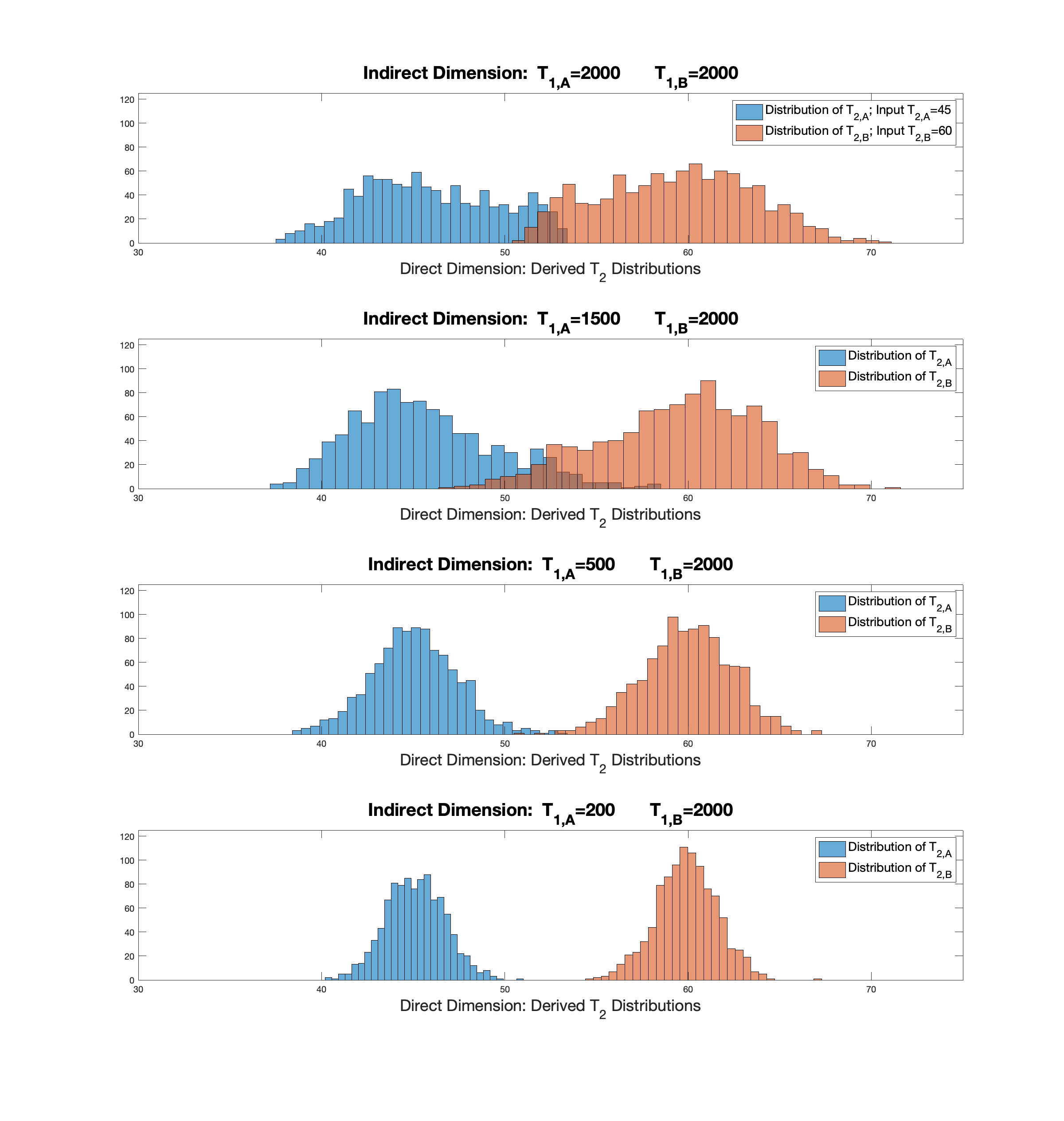
Fig.1 shows variances for recovery of $$$c_A,c_B,T_{2,A}$$$ and $$$T_{2,B}$$$ as a function of $$$T_{1,B}$$$ for the indicated example, with fixed $$$T_{1,A}=1000\hspace{2pt}ms$$$. All parameters show maximum error for $$$T_{1,B}=1000\hspace{2pt}ms$$$, with errors decreasing as $$$T_{1,B}$$$ deviates from this value. This result, based on the theory outlined above, is the major finding of this work, indicating the statistical basis for our previous empirical findings⁵ .

Fig.2 shows a Monte Carlo demonstration of the theoretical results. Histograms of fitted values over 1001 noise realizations are shown. There is a decrease in the variances of fitted values for T₂'s as the discrepancy between $$$T_{1,B}$$$ and $$$T_{1,A}$$$ increases in fits to the 2D model.

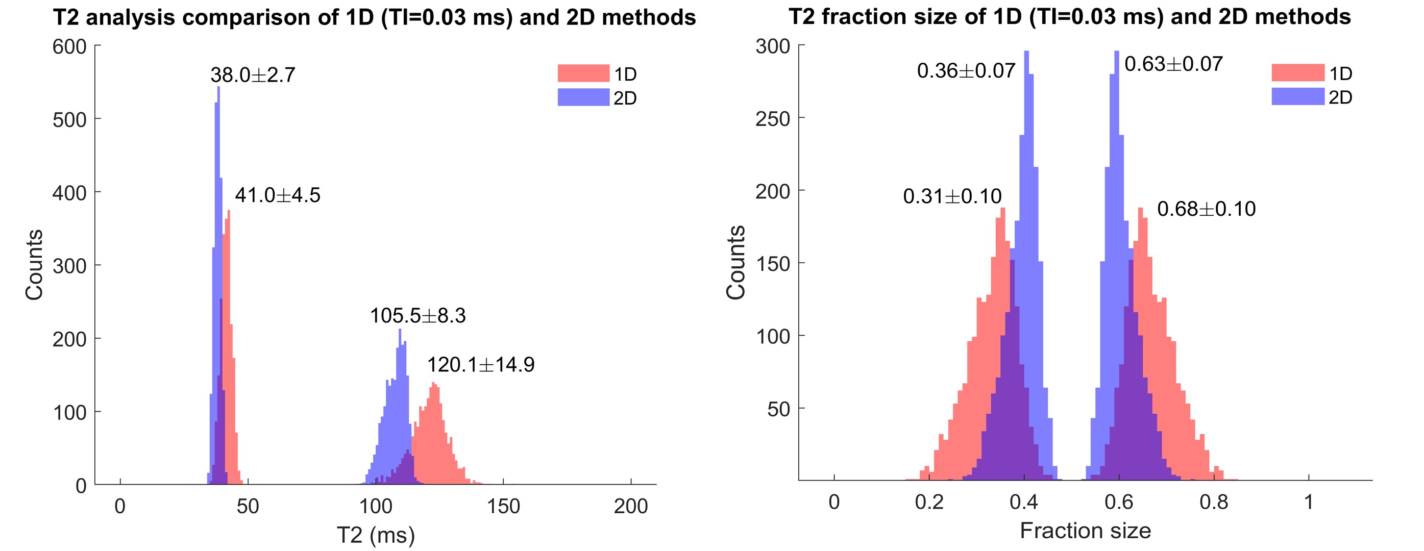
Fig.3 shows experimental results. Fitted parameter values across a uniform gel were used as a surrogate for noise realizations. Left: Histograms displaying fitted values of $$$T_{2,A}$$$ and $$$T_{2,B}$$$ over 1881 pixels; Right: fitted values of $$$c_A$$$ and $$$c_B$$$. The variance in fitted values is substantially smaller in the 2D as compared to the 1D experiment. This agrees with the theoretical (Fig.1) and simulation (Fig.2) results.

Discussion

MR relaxometry and diffusion experiments present difficult parameter estimation problems, with results highly dependent upon experimental noise. There is currently a great deal of interest in extending these experiments to higher dimensions. We have studied the statistical properties of these experiments and found that parameter estimation in higher dimensional experiments exhibits markedly improved stability, further increasing their significance.

Conclusion

Implementation of higher dimensional relaxometry provides a means of circumventing conventional limits on multiexponential parameter estimation. Further, all these results have been extended to the 3D and higher dimensional cases.

Acknowledgements

This work was supported entirely by the Intramural Research Program of the NIH National Institute on Aging.