3802
Faster Myelin water mapping by joint reconstruction and estimation from highly undersampled 3D-MSE acquisitions.1Department of Radiology and Nuclear Medicine, Erasmus Medical Center, Rotterdam, Netherlands
Synopsis
Myelin water fractions (MWF) can provide biomarkers for many brain disorders. Multiple-spin-echo (MSE) is considered as gold standard for obtaining MWF. However, its clinical application is limited by its long acquisition time. Efficient undersampling and exploiting the redundancy in the contrast images of MSE can decrease the acquisition time. We propose a subspace based image reconstruction technique designed for reconstructing contrast images from highly undersampled MSE acquisition, so that it can be used for MWF mapping. We evaluate it for different signal-to-noise ratios for up to acceleration factor of 16 and show its feasibility for accelerating acquisition beyond parallel imaging.
Introduction
Myelin water fractions (MWF) can provide biomarkers for diseases such as multiple sclerosis, schizophrenia, phenylketonuria and Alzheimer's 1-3. Multiple-spin-echo (MSE) is considered as benchmark for obtaining MWF and has been proven to be reproducible 3, 4. However, its clinical application is limited by its long acquisition time3.In MSE, much of the information in the contrast images is redundant. Recently, some techniques have been proposed to exploit this type of redundancy in the temporal dimension for reducing the acquisition time 5- 7. Joint reconstruction and parameter estimation (JRPE) has the potential to accelerate the acquisition of MSE beyond the acceleration factor (AF) permitted by parallel imaging. MWF extraction requires multi-exponential fitting which is badly conditioned unless a constrained fitting approach such as Non-negative least square (NNLS) fitting is applied1. Implementing such constraint is difficult in a JRPE framework.
Hence, we propose a subspace constrained image reconstruction technique to generate the contrast images from an undersampled acquisition. We generate a subspace using singular value decomposition (SVD) similar to Hamilton et al.8, but instead of using an MR fingerprinting dictionary we use the set of decays shown by each $$$T_2$$$ component in the multi-exponential model. Subsequently the MWF is estimated using the NNLS approach 1, 9. The dependence of the proposed method on subspace dimensionality as well as SNR is evaluated for AF up to 16.
Method
Signal modelLet the expected value for a k-space measurement in the 3D-MSE be $$$\mu_{j, \boldsymbol{k}, c}$$$ , where $$$j$$$ is index for different echoes ($$$j \in [1, J]$$$), $$$\boldsymbol{k}$$$ is a vector indexing multi-dimensional k-space ($$$\boldsymbol{k} \in \Omega_{\boldsymbol{k}} $$$) and $$$c \in [1, c_n]$$$ is coil index for coil with $$$c_n$$$ channels:
$$\mu_{j, \boldsymbol{k},c} =U_{j, \boldsymbol{k}} \sum_{ \boldsymbol{x} \in \Omega_{\boldsymbol{x} }} F_{ \boldsymbol{k}, \boldsymbol{x}} C_{\boldsymbol{x},c} S_{j, \boldsymbol{x}}, (1) $$
where $$$\boldsymbol{x}$$$ is a vector indexing multi-dimensional image domain $$$\boldsymbol{x} \in \Omega_{\boldsymbol{x}} $$$, $$$U_{j, \boldsymbol{k}} \in \{0, 1\}$$$ is the undersampling mask, $$$F_{ \boldsymbol{k}, \boldsymbol{x}} $$$ is Fourier operator, $$$C_{\boldsymbol{x},c}$$$ is coil sensitivity map and $$$ S_{j, \boldsymbol{x}}$$$ are the voxels from the contrast images. In a multi-exponential model 2, the signal from a single voxel in MSE can be modelled as,
$$ S_{j,\boldsymbol{x}} = \sum_{t=1}^{nT_2} s_{t,\boldsymbol{x}} e^{\frac{-{TE_t}}{T_{2,t}}}, (2)$$
where $$$nT_2$$$ is the number of logarithmically spaced $$$T_2$$$ times within an appropriately selected range, indexed by $$$ t \in [1, nT_2]$$$, $$$s_t$$$ is the unknown amplitude of the spectral component at relaxation time $$$T_{2,t}$$$ and $$$TE_t$$$ is the echo time.
Subspace reconstruction
The set of decays predicted by extended phase graph for each of $$$nT_2$$$ components were computed using the derivative of the model in equation (2), which is given by:
$$ D_{j,t} = \frac{ \partial S_{j,\boldsymbol{x}}}{ \partial s_{t,\boldsymbol{x}} } = e^{\frac{-{TE_t}}{T_{2,t}}}. (3)$$
$$$D_{j,t}$$$ is subjected to SVD and $$$d$$$ components were used for reconstructing contrast images by fitting. Finally, the $$$T_2$$$ distribution and subsequently MWF maps were obtained by applying NNLS fitting9 to the reconstructed contrast images.
Other acquisition settings
The main acquisition settings were taken from 4 in our simulation experiments: $$$J = 32$$$, echo spacing of $$$10$$$ ms , first echo time $$$TE1 = 10$$$ ms and $$$TR = 1000$$$ ms. As proposed in 10, $$$U_{j,\boldsymbol{k}}$$$ is generated with a Halton sequence to obtain a low discrepancy sampling scheme. The coil sensitivity map $$$C$$$ were obtained by ESPIRIT technique implemented in the BART toolbox from an acquisition with an 8-channel coil 11, 12.
Experiment
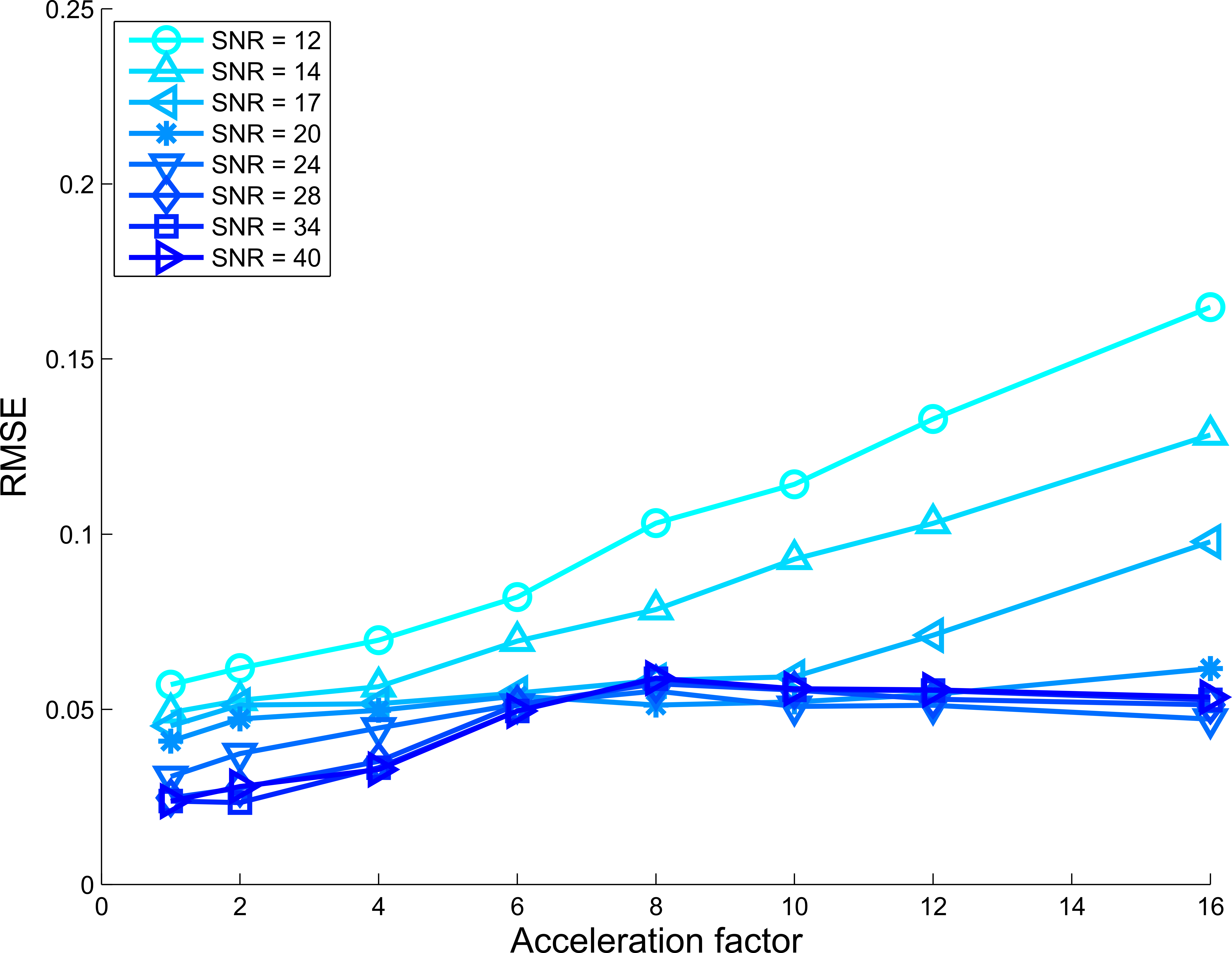
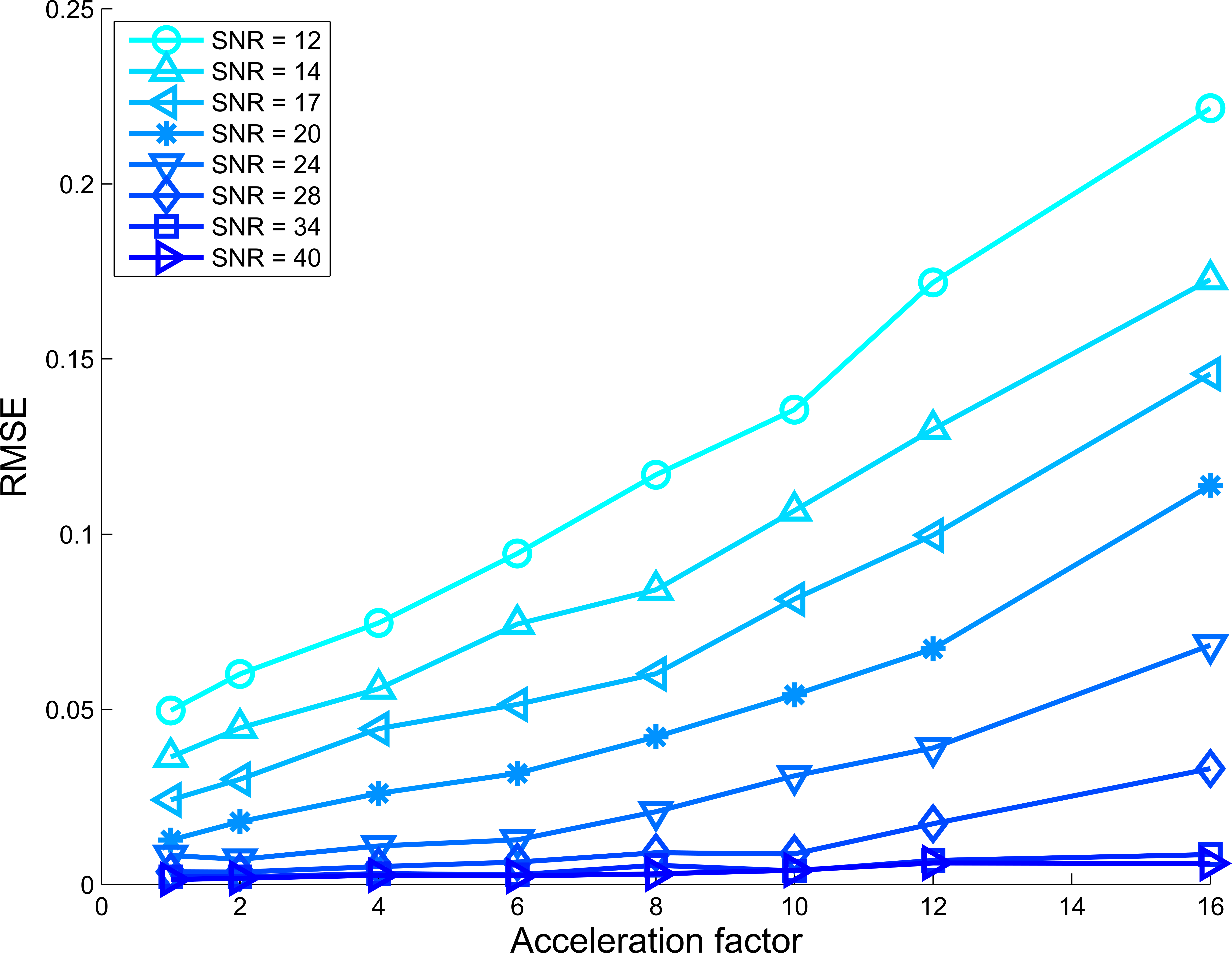
Figure 1 shows the two $$$T_2$$$ distributions (left) and the checkerboard pattern (right) that were used as the ground truth. Complex Gaussian noise was added to the signal model in equation (1) for acceleration factors (AF) of $$$1,2,4,6,7,10,12$$$ and $$$16$$$.The noise level was chosen to obtain 8 SNRs logarithmically placed between 12 and 40. The subspace reconstruction was performed with $$$d = 5,6,$$$ and $$$7$$$ components. The root mean square error (RMSE) was computed for each AF and SNR with respect to the ground truth MWF map.
Results
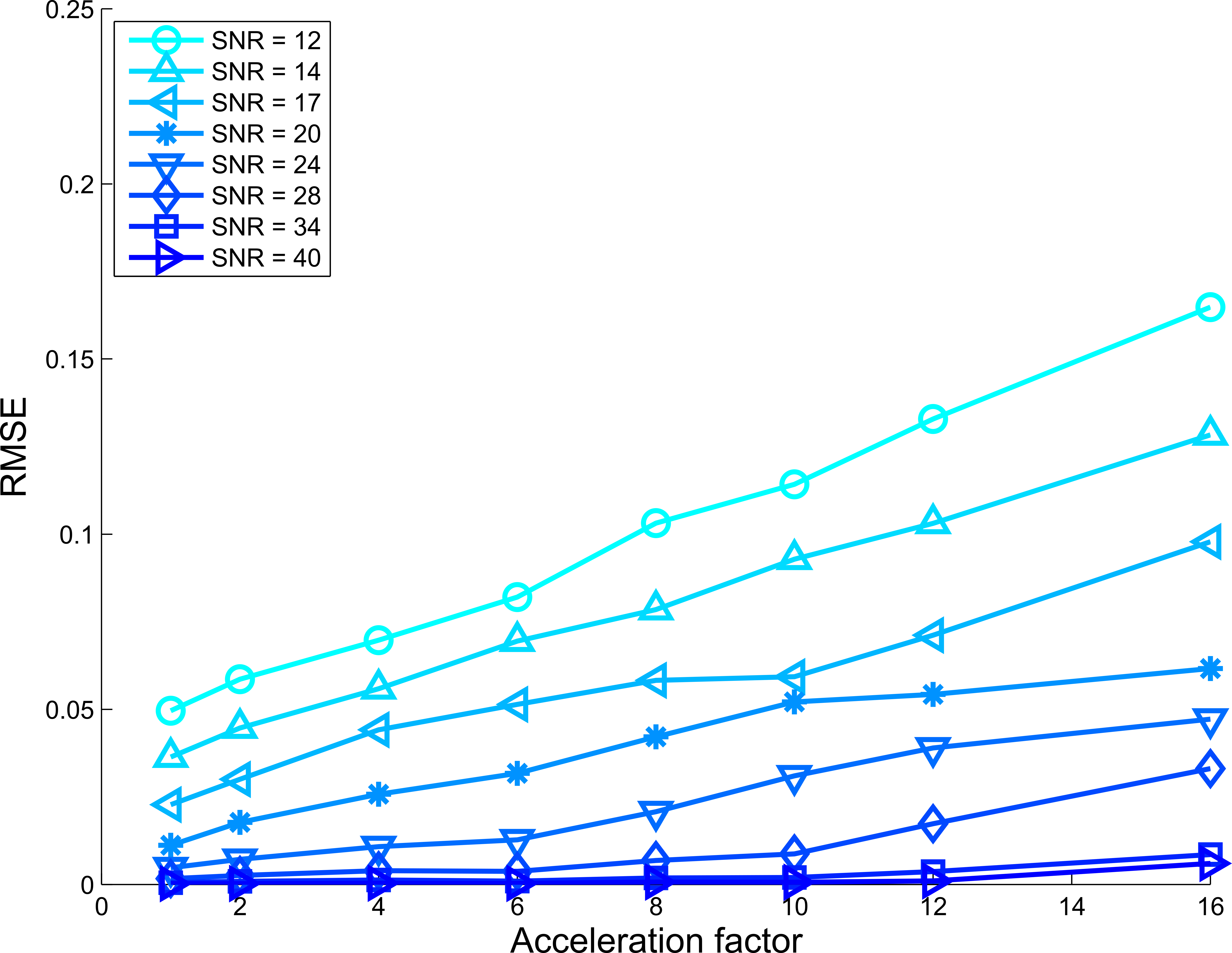
Figures 2, 3, and 4 show RMSE for all AFs and SNRs, for $$$d$$$ = $$$5,6$$$ and $$$7$$$ subspace components respectively. For the low SNR situation, using 5 subspace components gave the lowest RMSE. However, for high SNR the 6 components gave the lowest RMSE, where especially for high acceleration factors strong improvement was observed.Figure 5 shows lowest RMSE observed for all AFs and SNRs among all $$$d$$$ considered. SNR cases with SNR>12 and higher acceleration have lower RMSE than lower SNR cases upto specific AFs. For instance, the RMSE observed for AF=16 and SNR=28 was lower than the fully sampled case of SNR = 14.
Discussion
The optimal choice of $$$d$$$ depends on the SNR. The choice of numerical ground truth allows us to compute RMSE and take realistic distribution of $$$T_2$$$ and MWFs. The RMSE observed for accelerated acquisitions are comparable to the fully sampled cases of lower SNR, which shows that acceleration is feasible with acceptable increase in RMSE. This technique allows higher AFs than possible with parallel imaging.Conclusion
We show that proposed technique has the potential to accelerate the MSE acquisition for MWF mapping beyond the capability of parallel imaging using simulation.Acknowledgements
The authors would like to thank UBC MRI Research Centre for providing the code for NNLS fitting.
This work is part of project B-Q MINDED which has received funding from the European Union's Horizon 2020 research and innnovation programme under the Marie Sklodowska-Curie grant agreement No 764513.
References
1. A. Mackay, K. Whittall, J. Adler, D. Li, D. Paty, and D. Graeb, “In vivo visualization ofmyelin water in brain by magnetic resonance,” Magnetic Resonance in Medicine, vol. 31,pp. 673–677, June 1994.
2. K. P. Whittall and A. L. MacKay, “Quantitative interpretation of NMR relaxation data,” Journal of Magnetic Resonance (1969), vol. 84, pp. 134–152, Aug. 1989.
3. E. Alonso-Ortiz, I. R. Levesque, and G. B. Pike, “MRI-based myelin water imaging: Atechnical review: MRI-Based Myelin Water Imaging,” Magnetic Resonance in Medicine,vol. 73, pp. 70–81, Jan. 2015.
4. S. M. Meyers, I. M. Vavasour, B. Mdler, T. Harris, E. Fu, D. K. Li, A. L. Traboulsee, A. L.MacKay, and C. Laule, “Multicenter measurements of myelin water fraction and geometric mean $$$T_2$$$ : Intra- and intersite reproducibility: Reproducibility of Multicomponent $$$T_2$$$,”Journal of Magnetic Resonance Imaging, vol. 38, pp. 1445–1453, Dec. 2013.
5. D. Ma, V. Gulani, N. Seiberlich, K. Liu, J. L. Sunshine, J. L. Duerk, and M. A. Griswold,“Magnetic resonance fingerprinting,” Nature, vol. 495, pp. 187–192, Mar. 2013.
6. J. I. Tamir, M. Uecker, W. Chen, P. Lai, M. T. Alley, S. S. Vasanawala, and M. Lustig, “$$$T_2$$$ shuffling: Sharp, multicontrast, volumetric fast spin-echo imaging: $$$T_2$$$ Shuffling,” Magnetic Resonance in Medicine, vol. 77, pp. 180–195, Jan. 2017.
7. B. Zhao, B. Bilgic, E. Adalsteinsson, M. A. Griswold, L. L. Wald, and K. Setsompop, “Simultaneous multislice magnetic resonance fingerprinting with low-rank and subspace modeling,”in 2017 39th Annual International Conference of the IEEE Engineering in Medicine and Biology Society (EMBC), (Seogwipo), pp. 3264–3268, IEEE, July 2017.
8. J. I. Hamilton, Y. Jiang, D. Ma, Y. Chen, W.-C. Lo, M. Griswold, and N. Seiberlich, “Simultaneous multislice cardiac magnetic resonance fingerprinting using low rank reconstruction,”NMR in Biomedicine, vol. 32, p. e4041, Feb. 2019.
9. T. Prasloski, B. Mdler, Q.-S. Xiang, A. MacKay, and C. Jones, “Applications of stimulatedecho correction to multicomponent $$$T_2$$$ analysis,” Magnetic Resonance in Medicine, vol. 67,pp. 1803–1814, June 2012.
10. R. Byanju, S. Klein, A. Cristobal-Huerta, A. H. J. Tamames, and D. Poot, “Study of key properties behind a good undersampling pattern for quantitative estimation of tissue parameters,”in Proc. Intl. Soc. Mag. Reson. Med. 27 (2019), 4540, 2019.
11. M. Uecker, P. Lai, M. J. Murphy, P. Virtue, M. Elad, J. M. Pauly, S. S. Vasanawala, andM. Lustig, “ESPIRiT-an eigenvalue approach to autocalibrating parallel MRI: Where SENSEmeets GRAPPA,” Magnetic Resonance in Medicine, vol. 71, pp. 990–1001, Mar. 2014.
12. M. Uecker, J. I. Tamir, F. Ong, Siddharth Iyer, J. Y. Cheng, and M. Lustig, “Bart: Version0.3.00,” Jan. 2016
Figures