3801

Constraints in Estimating the Proton Density Fat Fraction

Mark Bydder¹, Vahid K Ghodrati¹, Yu Gao¹, Matthew D Robson², Yingli Yang¹, and Peng Hu¹
¹UCLA, Los Angeles, CA, United States, ²Perspectum Diagnostics, Oxford, United Kingdom

Synopsis

The study evaluates four physically motivated constraints in the estimation of the proton density fat fraction (PDFF) based on the physics of magnetic resonance imaging. These were smooth fieldmap, smooth initial phase, nonnegative proton density and moderate $$$R2*$$$ values. Results show that constraints are effective at reducing standard deviation and bias.

Introduction

The study evaluates four physically motivated constraints in the estimation of the proton density fat fraction ($$$PDFF$$$). Least squares approaches were developed for constraining the parameters in PDFF quantification based on the physics of magnetic resonance imaging. These were smooth fieldmap, smooth initial phase, nonnegative proton density and moderate R2* values. Constraints were evaluated in terms of their influence on the bias and standard deviation of the estimated parameters using numerical simulations and in vivo data acquired on a combined MRI-radiotherapy device at 0.35 T.

Methods

The signal from a mixture of water and fat in a single voxel can be written as in Eq 1

[Eq 1] $$$b = WAxe^{iφ}$$$

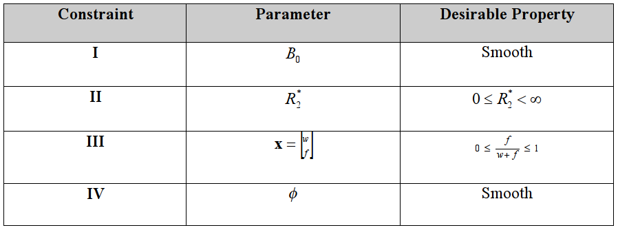
where $$$b$$$ is a vector of complex data points at $$$n$$$ echo times, $$$b$$$ is a vector of echo times, $$$A$$$ is an $$$n×2$$$ complex matrix expressing the evolution of water and fat, $$$W=diag(e^{iψt})$$$ is an $$$n×n$$$ matrix expressing the evolution of the complex fieldmap $$$ψ=B_0+iR_2^*$$$, $$$x=[w; f]$$$ is a real vector of water and fat proton densities and $$$φ$$$ is a real scalar (initial phase) [1]. The parameters of most clinical interest are $$$R_2^*$$$ and proton density fat fraction, $$$PDFF = f/(w+f)$$$ which can be obtained by iterative search over $$$B_0$$$, $$$R_2^*$$$, $$$x$$$ and $$$φ$$$ to minimize the residual norm $$$||r||$$$.

[Eq 2] $$$r=WAxe^{iφ}-b$$$

Since $$$B_0$$$ is a subject to $$$2π$$$ aliasing (fat-water swapping), a widely used strategy is to include a penalty term to encourage $$$B_0$$$ smoothness [2]. Since $$$B_0$$$ is also used to calculate susceptibility, it can be disadvantageous to compromise the resolution of $$$B_0$$$ [3] and thus it is of interest to consider alternative constraints. Table 1 lists some prior constraints that may be useful in solving the inverse problem. Previous work has shown there is a benefit to constraining Eq 1 [3-8], however to date there has been no systematic comparison of constraints using the same baseline methodology.

Results

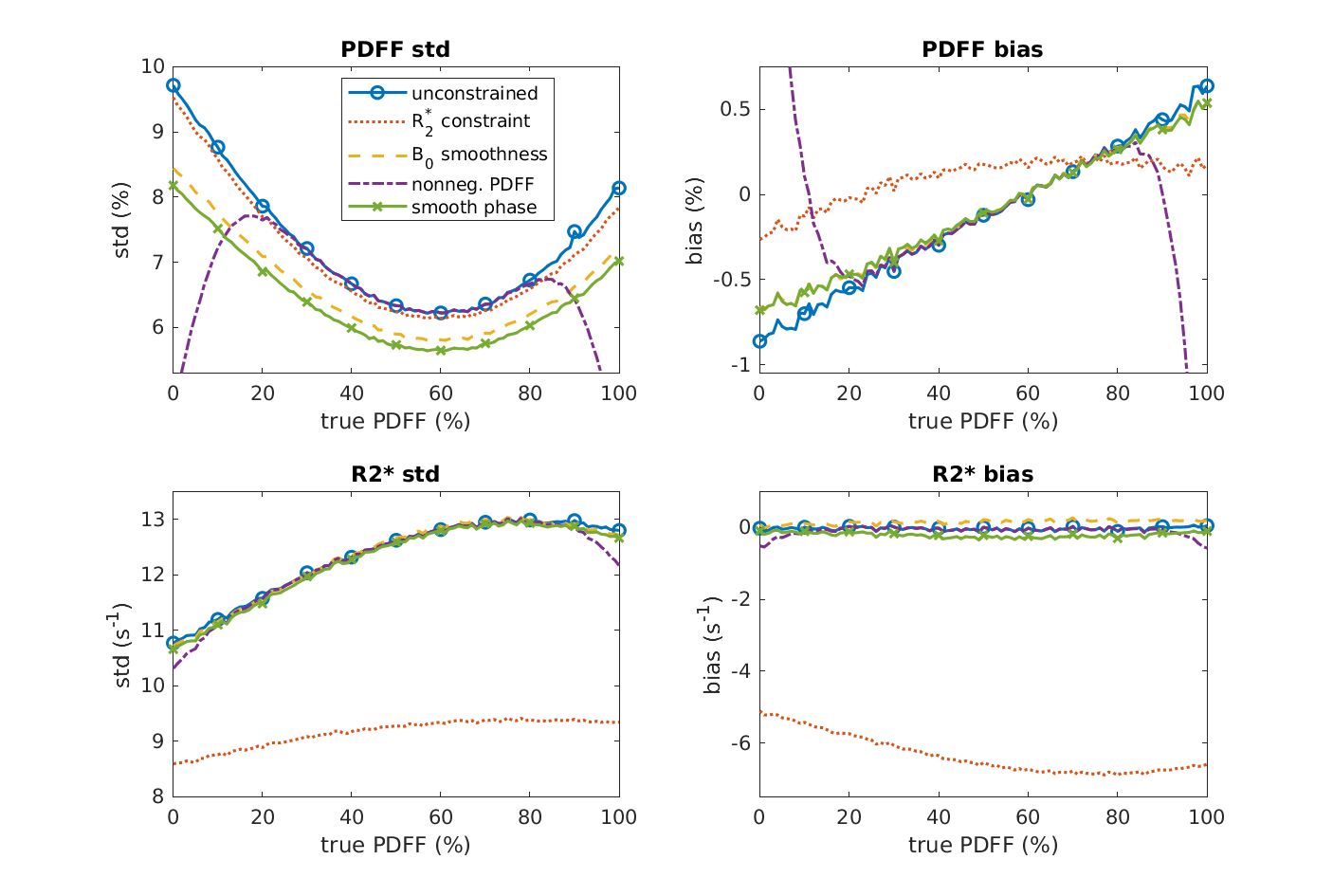
The constraints in Table 1 were implemented in a least squares minimization as described in [9]. Numerical simulations were performed using six echo times corresponding to (0.20π 0.56π 0.93π 1.30π 1.66π 2.03π). Multiple right hand side vectors ($$$b$$$ in Eq 1) were generated for $$$PDFF$$$ 0–100% with addition of complex Gaussian noise to give an SNR of 6 to reflect the typical situation at low field strength. Bias and standard deviation of the estimated $$$PDFF$$$ and $$$R_2^*$$$ were calculated over 10^5 trials to examine the effect of constraints.

Figure 1 shows simulation results of the standard deviation and bias (i.e. mean value – true value) over the range of $$$PDFF$$$ values. The top row is $$$PDFF$$$ and the bottom row is $$$R_2^*$$$. All of the constraints result in a reduction in standard deviation relative to unconstrained estimation. Constraint $$$I$$$ reduces the $$$PDFF$$$ standard deviation without any notable bias penalty other than sacrificing $$$B_0$$$ resolution). Constraint $$$III$$$ reduces the standard deviation of $$$R_2^*$$$ but also pulls the estimate toward zero (as may be expected). The standard deviation and bias of $$$PDFF$$$ are also reduced. Constraint $$$III$$$ has a strong influence at the end-points (as expected) with a large bias. Constraint $$$IV$$$ reduces the standard deviation with no notable effect on bias.

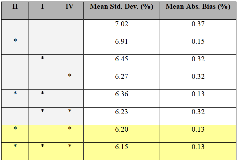
It is interesting to consider if constraints can be combined to achieve additive benefits. Unfortunately this does not not appear to be the case; key examples are given in Table 2. These indicate that Constraints $$$I$$$ and $$$IV$$$ both decrease the standard deviation but their combination is no better than the individual effects. Since it is a relatively unimportant parameter, the latter (smoothing the initial phase) may be a useful alternative to smoothing $$$B_0$$$.

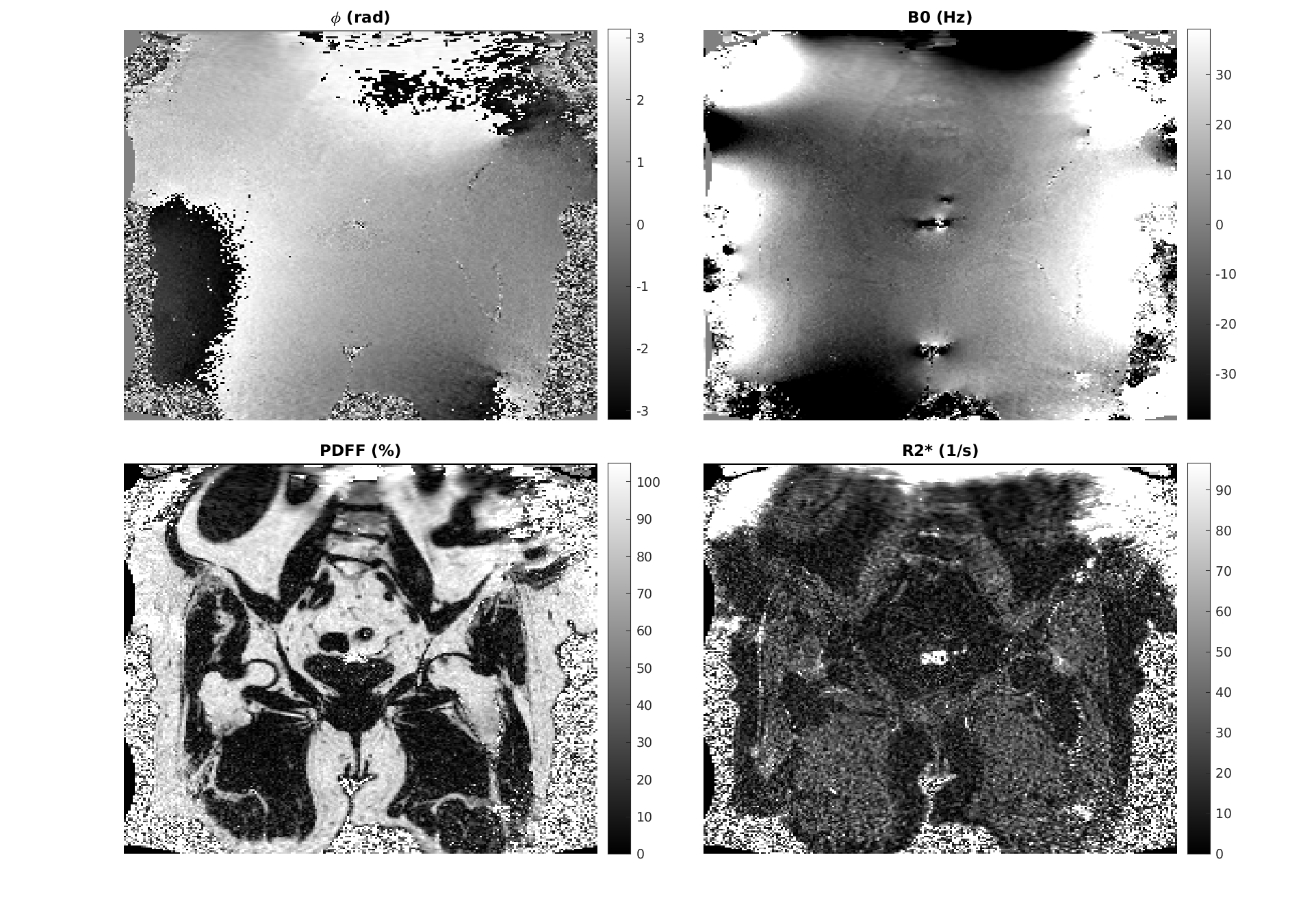
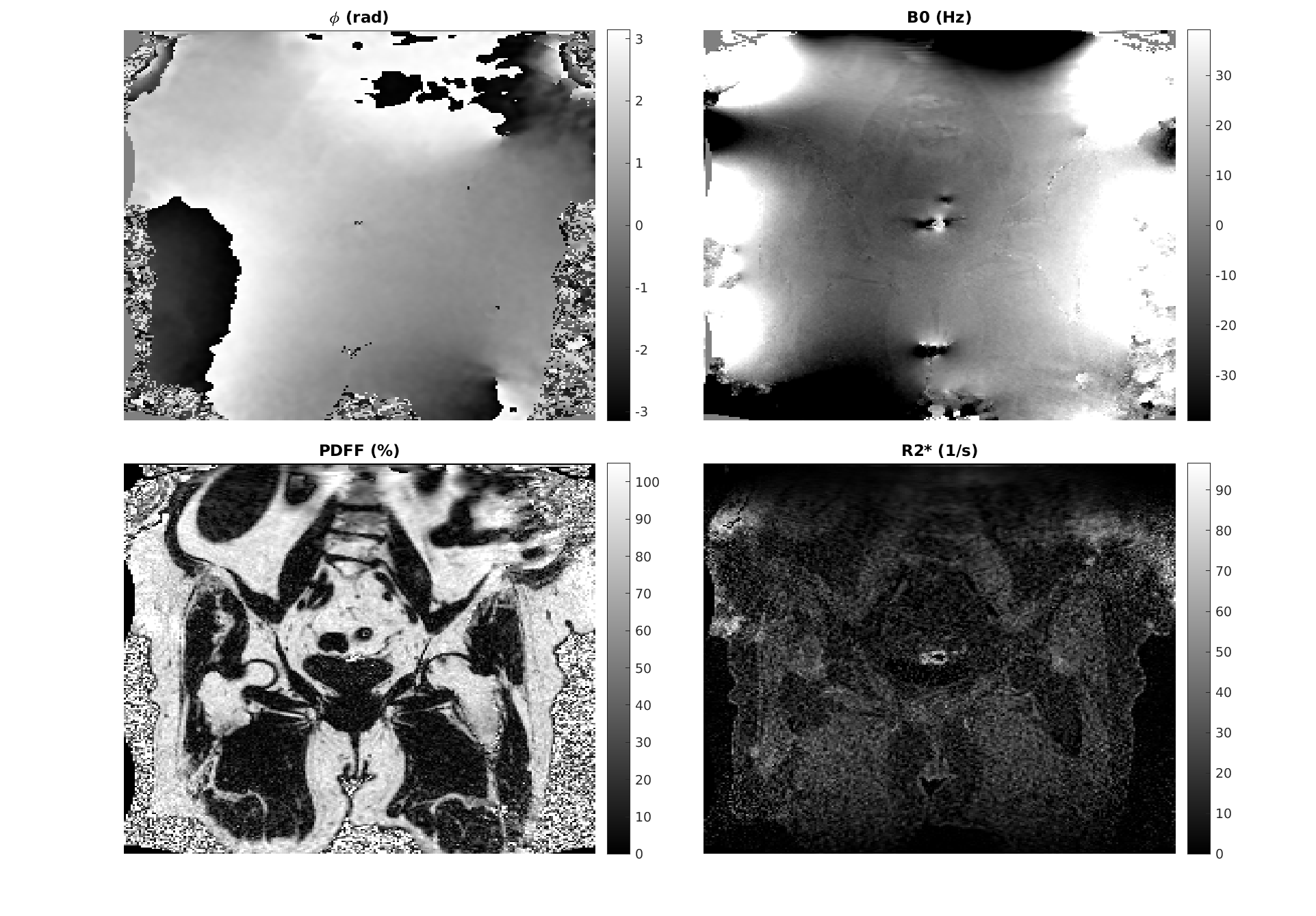
Figures 2 and 3 show in vivo results for unconstrained and constrained estimation (using Constraints $$$II$$$ and $$$IV$$$ only). The initial phase map differs in smoothness (as expected). The $$$B_0$$$, $$$R_2^*$$$ and PDFF maps all show a reduction in noise scatter and pointwise errors that occur in unconstrained fitting. The differences are small but in line with the anticipated effect size from simulations.

Discussion

Recent work has shown that $$$PDFF$$$ can be biased in noisy datasets [4,10,11], which is a challenge for estimation in the crucial low $$$PDFF$$$ range [12]. While it is desirable to reduce the bias and standard deviation, in general the two can only be traded against eachother with modeling choices. As shown in Figure 1, putting constraints on the parameters can provide a mechanism to manipulate bias and standard deviation. Furthermore, certain choices of constraints reduce both the bias and standard deviation of the $$$PDFF$$$ estimate.

Acknowledgements

No acknowledgement found.

References

[1] M Bydder, T Yokoo, H Yu, M Carl, SB Reeder, CB Sirlin. Constraining the initial phase in water-fat separation. Magn Reson Imaging 2011; 29: 216-221

[2] D Hernando, JP Haldar, BP Sutton, J Ma, P Kellman, ZP Liang. Joint estimation of water/fat images and field inhomogeneity map. Magn Reson Med 2008; 59: 571-580

[3] A Karsa, S Punwani, K Shmueli. The effect of low resolution and coverage on the accuracy of susceptibility mapping. Magn Reson Med 2019;81:1833

[4] Liu CY, McKenzie CA, Yu H, Brittain JH, Reeder SB. Fat quantification with IDEAL gradient echo imaging: correction of bias from T1 and noise. Magn Reson Med 2007;58:354

[5] SD Sharma, HH Hu, KS Nayak. Accelerated T2*-Compensated Fat Fraction Quantification Using a Joint Parallel Imaging and Compressed Sensing Framework. J Magn Reson Imag 2013; 38: 1267

[6] H Yu, SB Reeder, CA McKenzie, ACS Brau, A Shimakawa, JH Brittain, NJ Pelc. Single acquisition water fat separation: Feasibility study for dynamic imaging. Magn Reson Med 2006; 55: 413

[7] Lu W, Hargreaves BA. Multiresolution field map estimation using golden section search for water-fat separation. Magn Reson Med 2008;60:236–244

[8] J Andersson, H Ahlström, J Kullberg. Water-fat separation incorporating spatial smoothing is robust to noise. Magn Reson Imag 2018; 50: 7

[9] M Bydder, VG Kouzehkonan, Y Gao, MD Robson, Y Yang, P Hu. Constraints in Estimating the Proton Density Fat Fraction. Magn Reson Imaging 2019 (in press)

[10] NT Roberts, D Hernando, JH Holmes, C Wiens, SB Reeder. Noise properties of proton density fat fraction estimated using chemical shift-encoded MRI. Magn Reson Med 2018; 80: 685-695

[11] CW Hong, G Hamilton, C Hooker, CC Park, CA Tran, WC Henderson, JC Hooker, SF Dehkordy, JB Schwimmer, SB Reeder, CB Sirlin. Measurement of spleen fat on MRI-proton density fat fraction arises from reconstruction of noise. Abdominal Radiology 2019; 44: 3295

[12] EM Petäjä, H Yki-Järvinen. Definitions of Normal Liver Fat and the Association of Insulin Sensitivity with Acquired and Genetic NAFLD—A Systematic Review. Int J Mol Sci 2016; 17: 633

Figures

Table 1: The unknown parameters in Eq 1 and the physical properties that may be useful to constrain the estimation problem.

Figure 1: Simulation results of the PDFF (top row) and $$$R_2^*$$$ (bottom row) for unconstrained estimation and for the individual constraints listed in Table 1. The main influences on PDFF standard deviation are the two smoothness constraints whereas the main influence on $$$R_2^*$$$ is the associated constraint. In the $$$R_2^*$$$ bias plot, there is little effect of constraints except the $$$R_2^*$$$ constraint which biases the result towards zero.

Table 2: The effect of combining constraints, as assessed by the mean standard deviation and mean absolute bias in $$$PDFF$$$. The marker (*) indicates the constraint was active. Note that Constraint III was excluded since it causes excessive bias in the low range. Overall the standard deviation typically decreases as more constraints are used but is not a simple accumulation of the individual constraints. The best performance is with all constraints active (bottom row) however this includes $$$B_0$$$ smoothing; the next best is the second from bottom row.

Figure 2: In vivo results using unconstrained estimation. There are numerous point-wise errors since the voxels are essentially fitted independently and does not exploit spatial smoothness properties in any of the parameters.

Figure 3: The same data as Figure 2 using the Constraints II and IV. The phase is smoother than in Figure 2 and many of the point-wise errors are gone. The $$$B_0$$$, $$$PDFF$$$ and $$$R_2^*$$$ all exhibit a reduction in noise scatter compared to unconstrained estimation. Based on simulations, the anticipated effect size should be on the order of a 5 % reduction in standard deviation.

Proc. Intl. Soc. Mag. Reson. Med. 28 (2020)

3801