Introduction:

In the standard-of-care setting, great emphasis is placed on collecting dynamic contrast-enhanced MRI (DCE-MRI) data at very high spatial resolution, thereby necessitating low temporal resolution (e.g., 60-120 sec). This precludes accurate quantification of pharmacokinetic parameters that are important indicators of malignancy, and does not allow tracking of the contrast media bolus as it propagates through arteries and veins. We have previously developed novel image processing and computational modeling methods^1,2 to characterize tumor-associated vessels to assist in the diagnosis of suspicious breast lesions. Specifically, we have developed algorithms to automatically segment the breast vasculature in 3D, identify individual tumor feeding and draining vessels, and compute vessel number and tortuosity¹. Furthermore, we developed an image-based computational fluid dynamics model to characterize the blood supply and interstitial transport associated with individual lesion². Now we employ a dynamic digital phantom to systematically and rigorously determine an optimal acquisition-reconstruction protocol that balances acquisition demands with clinical reality, thereby enabling quantitative hemodynamic analysis to be widely available for the characterization of cancer.

Methods:

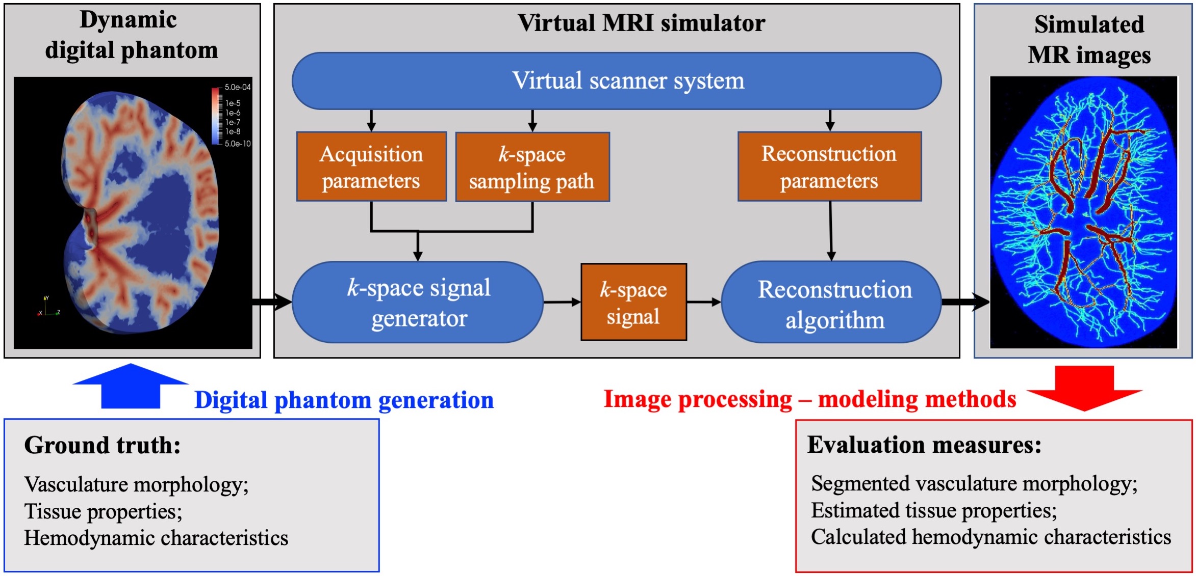
The overall workflow is illustrated in Figure 1. We first generate the dynamic digital phantom using ultra-high-spatial resolution data³ collected in an excised rat kidney. The highly structured vascular network is extracted from the kidney images, and realistic values for MR properties (e.g., longitudinal/transverse relaxation time, proton density) and physiological properties (e.g., vascular permeability, tissue conductivity) are assigned to the vascular and extravascular tissue. Detailed methods and results of the digital phantom generation can be found in another abstract submitted to ISMRM 2020 [Abstract #2822]. The morphology of the vasculature and the assigned tissue properties and hemodynamics are considered as the “ground-truth” in the simulations that follow.
We adapt the virtual MRI simulator developed by Easley et al.^4,5 to simulate virtual MR images based on the theoretical signal equations of DCE-MRI corresponding to specific acquisition parameters, k-space sampling paths, and reconstruction parameters. The simulator produces a realistic, continuous change of the “ground truth” over time due to contrast agent perfusion. Importantly, this means the signal at every point in the k-space represents the dynamic status of the digital phantom at the specific time when this point is sampled. Thus, a reconstruction can be achieved with much higher temporal resolution (e.g., 250 ms/frame) than the nominal scan time (3.5 s/scan) by optimizing over a regularized temporal smoothing constraint via gradient descent. We then add noise and downsample these high resolution, high SNR images and reconstruct to produce virtual MR images with varying spatial resolution, temporal resolution, and SNR. The resulting DCE-MRI data sets are then subjected to our analysis^1,2, to recover estimates of the vascular network, pharmacokinetic parameter estimation, and image-guided computational fluid dynamic modeling². The outputs are then compared to the “ground truth”, so that the dependence of the analysis on data quality (i.e., temporal/spatial resolutions, SNR) can be systematically determined.

Results:

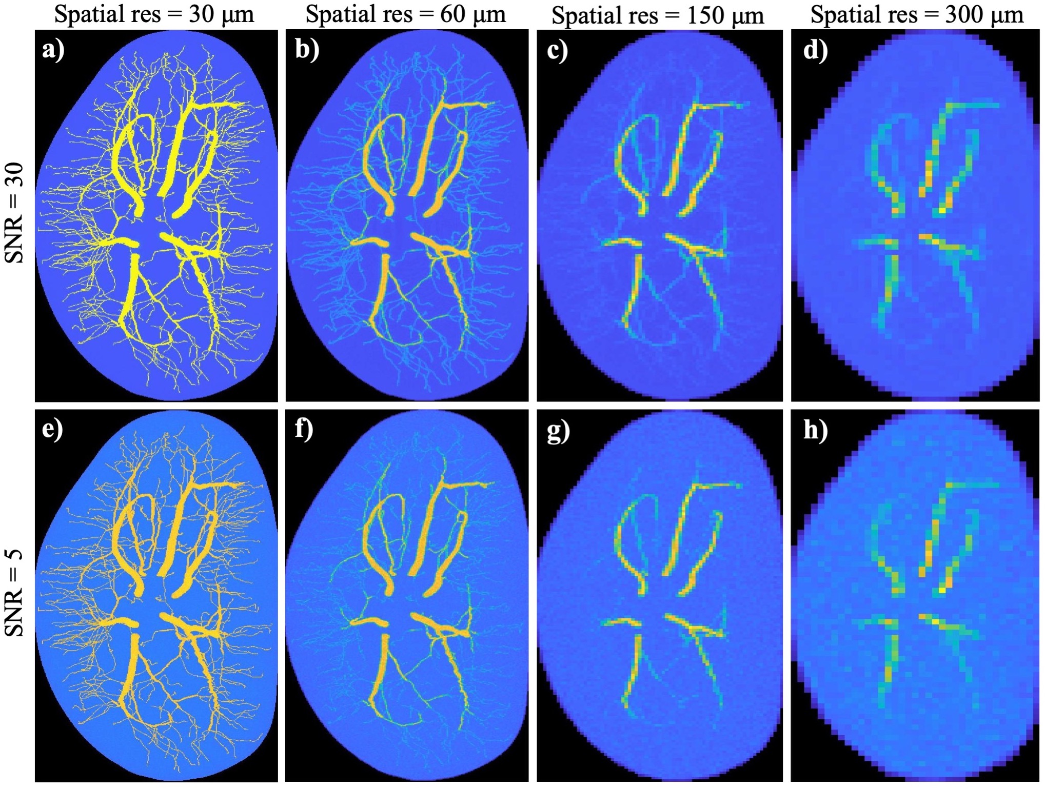
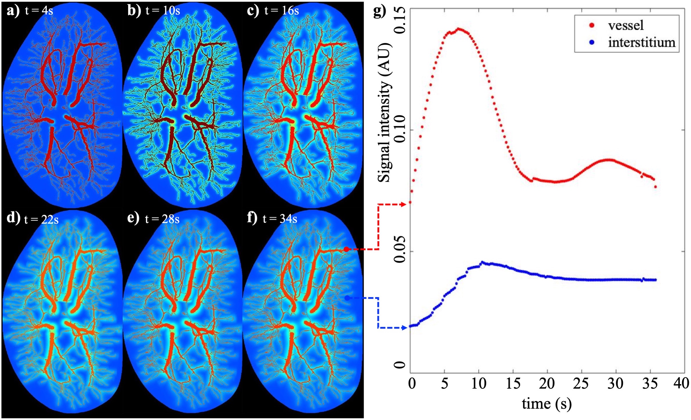
Figure 2 shows the simulated MR images from the first time point obtained with varying combinations of spatial resolution and SNR. The images in first and second rows are generated with an SNR = 30 and 5, respectively. Images in the first column are generated with the same spatial resolution as the original digital phantom (i.e., 30 μm). The remaining three columns from left to right are reconstructed at spatial resolution reduced by a factor of 2, 5 and 10, respectively, (i.e., spatial resolution of 60 μm, 150 μm, and 300 μm). Observation indicates that the contrast of micro-vasculature to the background are significantly affected by both the down-sampling and increasing of noise, with contrast-to-noise ratios (i.e. ratio of the median in vessel ROIs to the standard deviation in non-vessel ROIs) equal 174.95, 16.99, 10.29, 6.90 for SNR = 30 and spatial resolution of 30, 60, 150 and 300 μm respectively, and equal 21.49, 9.47, 7.36, 5.65 for SNR = 5 and spatial resolution of 30, 60, 150, and 300 μm.
Figure 3 shows the time series of simulated images and the corresponding time courses for example voxels. The reconstructed images in panels (a)-(f) show the change in spatio-temporal distribution of the contrast agent, revealing the dynamics of perfusion, interstitial convection, and diffusion. Panel (g) shows the time courses associated with example vascular (red) and extravascular (blue) voxels. The ultrafast reconstruction with 250 ms temporal resolution is able to capture the peak of bolus profile.

Discussion and Conclusions:

We have established a novel workflow to systematically evaluate quantitative DCE-MRI analysis methods using a dynamic digital phantom and simulation of virtual MRI data. We have used the digital phantom to generate dynamic MRI data with varying resolutions and SNR. We are now working on applying the analysis methods^1,2, including the vasculature segmentation, and the estimates of tissue properties and hemodynamics characteristics, on the simulated images. A major challenge in our current implementation is the reconstruction algorithm involves solving a large linear system, which is very memory- and time-intensive, with above 500 GB memory required and hours for computation to converge. We are currently working to parallelize the analysis to significantly improve performance. We hope to use this dynamic phantom to optimize dynamic acquisition and reconstruction protocols to balance analysis demands within the restrictions of clinical imaging settings.

Acknowledgements

NCI U01CA142565, U01CA174706, and R01 CA218700. CPRIT RR160005. T.E.Y. is a CPRIT Scholar in Cancer Research. MR histology images courtesy of Duke Center for In Vivo Microscopy.