Introduction

Quantitative MRI (qMRI) has great potential as information about tissue parameters can provide meaningful indications of disease.^1-2 In particular, quantifying $$$T_{2}^{*}$$$ offers relatively time-efficient data acquisition and relatively low specific absorption rate (SAR).^3-4 However, it requires images acquired at a long echo time (TE) for an accurate quantification, which leads to an increased TR and scan time. Although parallel imaging reduces scan time, acceleration factors are limited as aliasing artefacts may corrupt $$$T_{2}^{*}$$$ quantification.⁵ To alleviate such problems, model-based reconstruction methods have been proposed for $$$T_{1}$$$ and $$$T_{2}$$$ mapping.^5-6 They directly estimated parameter maps together with proton density images from the undersampled k-space data using the forward signal model. In this work, this concept is extended to quantify $$$T_{2}^{*}$$$ values. The model-based reconstruction benefits from the large number of echoes which can be acquired in multi-echo gradient echo (GRE) acquisitions. The proposed method provides accurate $$$T_{2}^{*}$$$ maps as well as images reconstructed at every TE from highly undersampled data.

Methods

The model-based joint reconstruction and parameter estimation can be written as⁷:
$$\Theta=\operatorname{argmin}\sum_{t,k,c}\left|S_{t,k,c}-\mu_{t,k,c}\right|^{2}, {\quad}\text {where}{\,}{\,} \mu_{t,k,c}=U_{t,k} \sum_{x\in X} F_{k,x}\left(C_{x,c} f_{t}\left(\boldsymbol{\theta}_{x}\right)\right),{\quad}{Eq. 1}$$ where $$$S_{t,k,c}$$$ are the acquired k-space data, $$$t$$$, $$$k$$$, and $$$c$$$ are indices for echo number, k-space position, and coil element, respectively. $$$\mu_{t,k,c}$$$ are the predicted data, $$$U_{t,k}$$$ is the undersampling pattern, $$$F_{k,x}$$$ is the Fourier transform operator, $$$x$$$ is the spatial position index, $$$C_{x,c}$$$ is the coil sensitivity, $$$f_{t}(\theta_{x})$$$ is a model function predicting the transversal magnetization of echo $$$j$$$ from the parameters vector $$$\theta_{x}$$$, $$$Θ$$$ is the collection of $$$\theta_{x}$$$vectors for all $$$x$$$.
For a multi-echo GRE sequence, $$$f_{t}(\theta_{x})$$$ was modelled by⁸:
$$f_{t}\left(\theta_{x}\right)=f_{t}\left(\rho_{w}, \rho_{f}, T_{2}^{*}, \phi_{off}, \phi_{0}\right)=\left(\rho_{w}+\rho_{f} \sum_{p=1}^{P} \alpha_{p}\mathrm{e}^{\mathrm{i}2\pi f_{p}TE_{t}}\right)\mathrm{e}^{\left(-\left(1/T_{2}^{*}+i\phi_{off}\right) TE_{t}-\phi_{0}\right)}$$ where $$$\rho_{w}$$$ and $$$\rho_{f}$$$ are proton densities of water and fat, $$$\phi_{off}$$$ and $$$\phi_{0}$$$ are off-resonance frequency and initial phase at TE = 0 respectively. The relative amplitude of the p^th fat peak, $$$\alpha_{p}$$$, with frequency shift $$$f_{p}$$$ is specified a priori.

A healthy subject was scanned at a 3T MR scanner (PRISMA, Siemens Healthineers, Erlangen, Germany) with a 20-channel head coil. A multi-echo GRE with bipolar readout gradients (QUTE)^9-11 was used: FOV=210×210mm², matrix =128×128, slice thickness=2mm, TR=600ms, #slices=3, #echoes=128, TE1=4ms, ∆TE=0.99ms, and 1302bw/px. The acquired datasets were fully sampled.

As a preprocessing step, linear phase differences between odd and even echoes (timing error) were corrected along the frequency encoding direction. An initial reconstruction was obtained by subspace constrained reconstruction.¹² A 21-dimensional subspace was calculated by SVD from a wide range of parameters, e.g., $$$T_{2}^{*}{\in}[5, 125]$$$, $$$\phi_{off}{\in}[-200, 200]$$$, and $$$\phi_{0}{\in}[-1/\pi, 1/\pi]$$$. Initial parameters were obtained by dictionary matching on the initial reconstruction. Subsequently, Eq. 1 was optimized by a trust-region dogleg method.

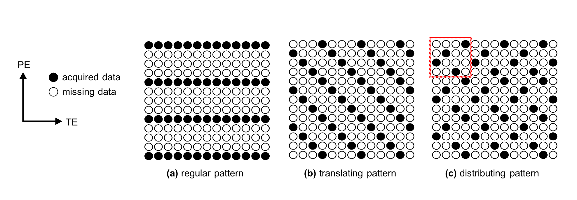
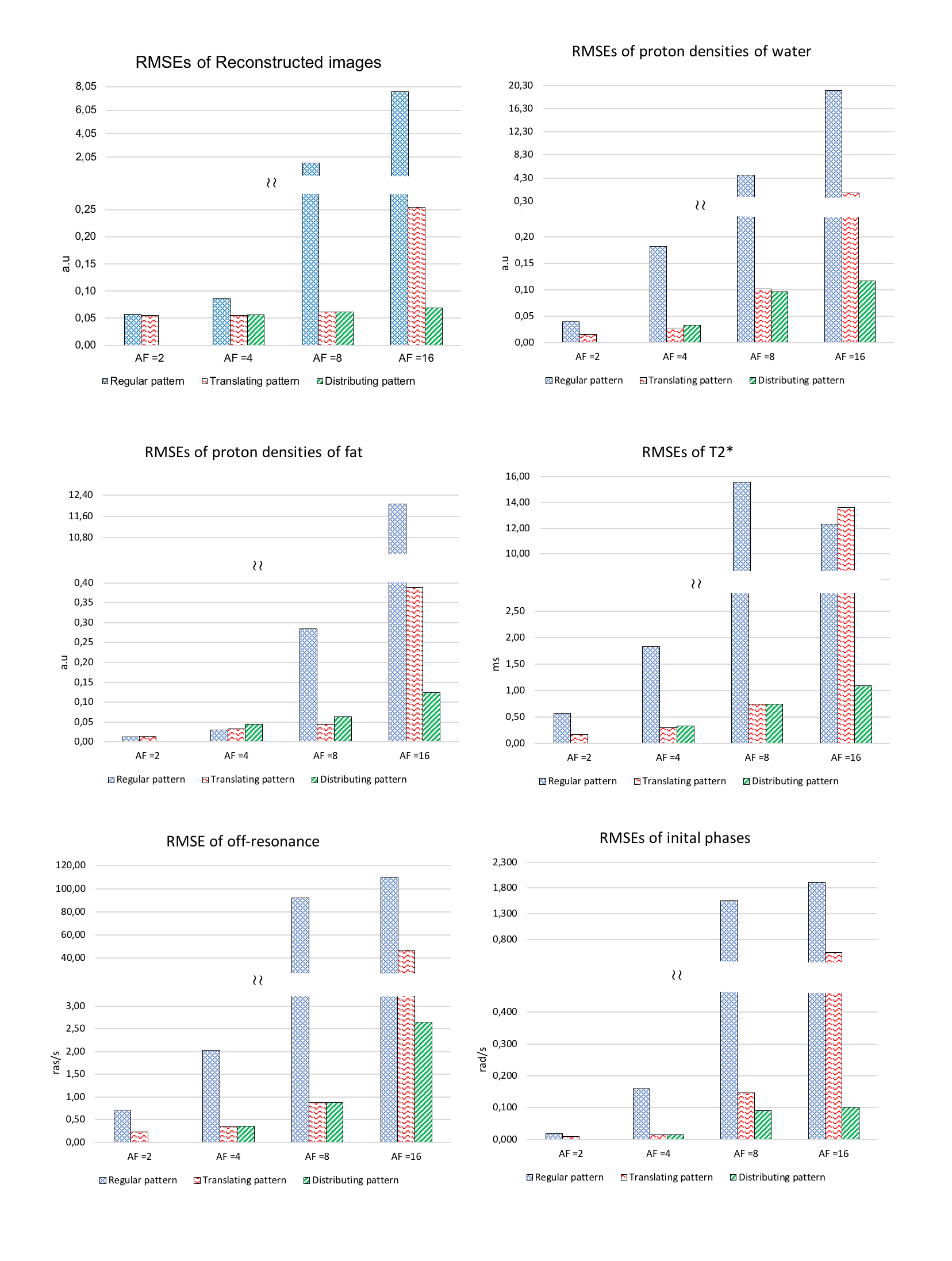
To validate the performance of the proposed method, datasets were retrospectively undersampled along the phase-encoding (PE) direction. The acceleration factor (AF) was increased from 2 to 16 in multiples of 2. For each AF except for AF 2, a total of three undersampling patterns were investigated (Fig. 1). Quantitative analyses were performed by comparing the root mean squared errors (RMSEs):
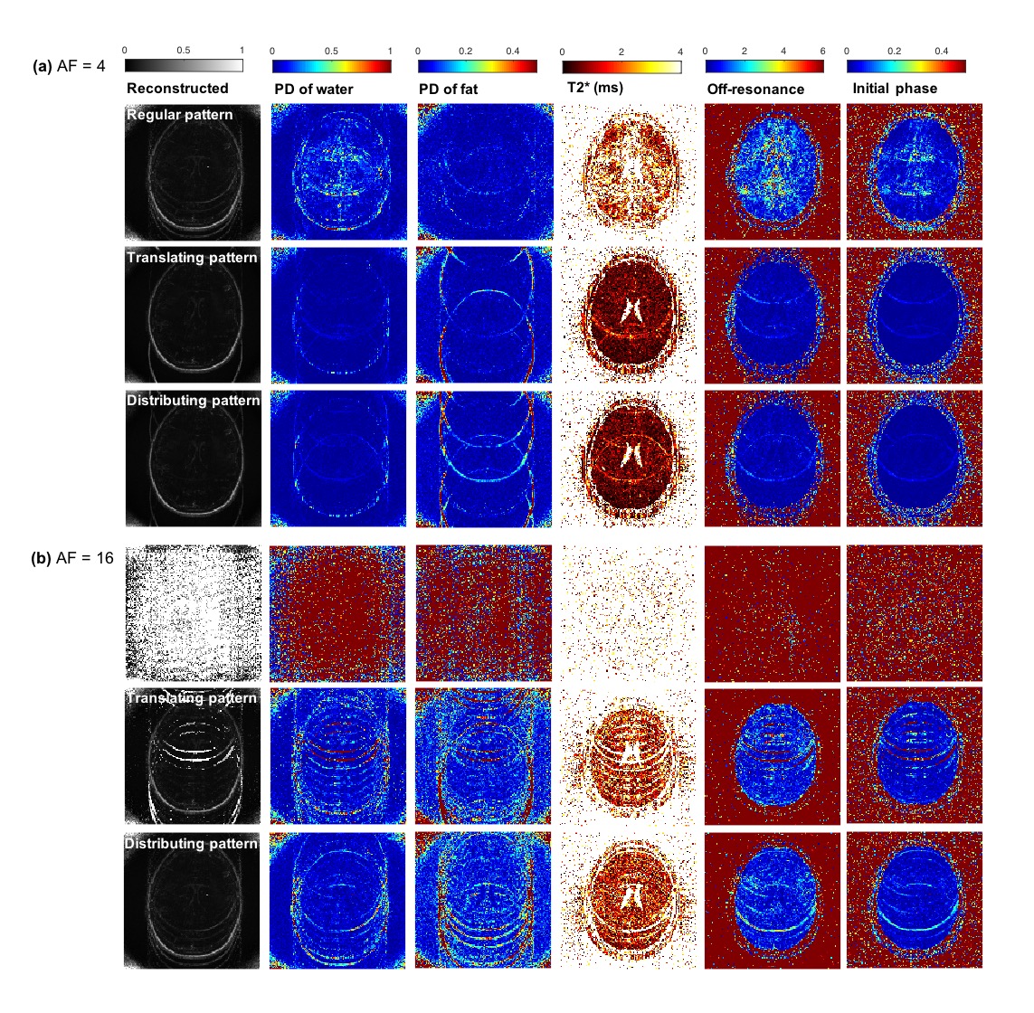
$$RMSE_{Img}=\sqrt{\frac{\sum_{ROI}\sum_{t=1}^{nTE}\left|I_{t}^{Full}-I_{t}^{Recon}\right|^{2}}{M*nTE}}$$ where $$$M$$$ is the number of voxels in brain region, $$$nTE$$$ is the number of echoes, $$$I_{t}^{Full}$$$ and $$$I_{t}^{Recon}$$$ are images with fully sampled k-space data and reconstructed images from undersampled k-space data, based on the estimated parameter maps, respectively. The RMSE was also computed directly on the estimated parameter maps: $$RMSE_{map}=\sqrt{\frac{\sum_{ROI}\left|map^{Full}-map^{Under}\right|^{2}}{M}}$$ $$$map^{Full}$$$ and $$$map^{Under}$$$ are estimated parameter maps from the fully sampled and undersampled k-space data, respectively.

Results

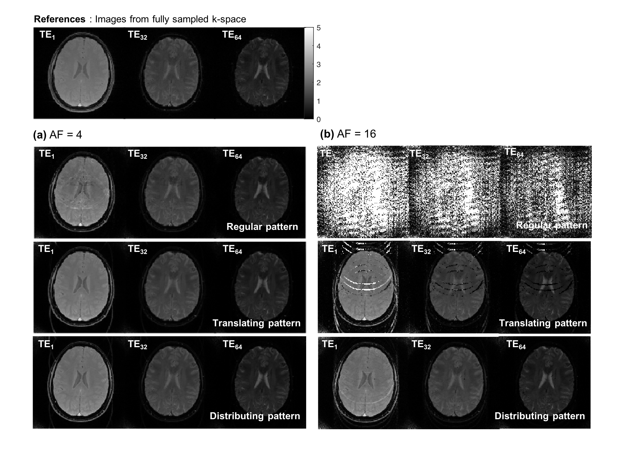
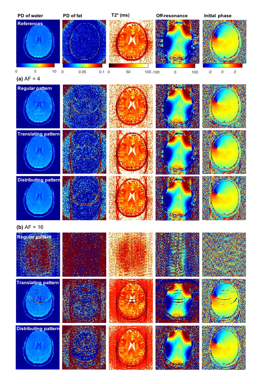
Figure 2 and 3 shows the reconstructed images and parameter maps from the undersampled k-space data. Fig. 2a, 3a and 2b, 3b are results from AF of 4 and 16 respectively. With the distributing pattern, the proposed method achieved good reconstructions even for the higher acceleration factors, although some aliasing artefacts were visible for acceleration factors 8 and 16. Figure 4 shows RMSE images from the reconstructed images and parameter maps. Figure 5 shows the RMSE in the brain for all AFs. The RMSE in $$$T_{2}^{*}$$$ of the distributing pattern at AF 16 was 1.6 times lower than that of regular AF 4, and only two times higher than that of regular AF 2.

Discussion

With the regular undersampling pattern, aliasing artefacts are significant beyond an acceleration factor of 2, indicating the limit of parallel imaging alone. With the translating, but especially the distributing undersampling pattern the model-based joint reconstruction and parameter estimation method enables increased acceleration factors. For these patterns, regular and for each TR equal blip gradients are needed in an actual implementation. Such prospective undersampling and investigation of eddy current effects are left for future work.

Conclusions

We validated that the joint reconstruction method allows quantifying $$$T_{2}^{*}$$$. It provided $$$T_{2}^{*}$$$ maps as well as the other parameter maps with an acceleration factor 16, without using prior information on image content or appearance. Such acceleration improves the feasibility of using $$$T_{2}^{*}$$$ quantification in clinical applications.

Acknowledgements

This work was supported by the European Union’s Horizon 2020 research and innovation programme under the Marie Sklodowska-Curie grant agreement No 764513.