Introduction

T₁ quantification enables the non-invasive characterization of tissue, providing relevant clinical information about the heart, the liver or even musculoskeletal regions.^1-4 Inversion Recovery sequences with balance Steady State Free Precession (bSSFP) readouts are often used to measure the T₁ parameter but this approach has been shown to be vulnerable to partial volume effects (PVE) which can arise from fat infiltration.^1-3 In addition, the fat effect on T₁ estimates may differ in the presence of static B₀ field inhomogeneities (ΔB₀).⁵ To improve the accuracy of the T₁ estimates, this information can be separately measured and taken into account in the fitting. ^1,6 An alternative method (FLASH), which relies on spoiled gradient echo readouts, is known to be more robust to ΔB₀ and can also be applied to T₁ mapping⁷, but the effect of fat in this context has not yet been studied. With this work, we evaluate the behaviour of T₁ mapping with MOLLI using FLASH readout (FLASH-MOLLI) in the presence of fat. In addition, we propose a new bi-component model which accounts for the existence of fat avoiding T₁ discrepancies due to PVE to both FLASH-MOLLI and bSSFP-MOLLI.

Methods

MOLLI signals using acquisition schemes: 5(3)3, 3(3)3(3)5, and 4(3)3(3)2 for an RR=1000ms, with a bSSFP (FA=35º,TI₁=100ms;TR/TE=2.5/1.25ms), and FLASH (FA=10º,TI₁=120ms; TR/TE=3.6/1.4ms) readouts were simulated in Matlab2016a. Signals representing pure myocardial (T₁/T₂=1000/50ms; on-resonance) and fat tissues (T₁/T₂=260/60ms; 430Hz off-resonance)³ were combined to mimic fat fractions (FF) of [0.00-0.50]. Gaussian noise was added to obtain a typical SNR=80 at 3T. For both bSSFP-MOLLI and FLASH-MOLLI signals, T₁ values were estimated with the conventional mono-component 3-parameter fitting ⁸ (Eq.1).
$$S_{MOLLI}^{mono-component}\left(t,A,B,T_{1}^{*}\right)=A-B\exp\left\{-t/T_{1}^{*}\right\} \mathbf{Eq}(1)$$

The proposed bi-component model which accounts for both fat and water within the pixel (Eq.2) was also applied. In this model if a pixel is composed of two species, the signal can be expressed as:

$$\text{Signal}=\sum_{i=1}^{2}A_{i}-B_{i}\exp\left\{-\frac{t}{T_{1i}^{*}}\right\}\mathbf{Eq}(2)$$
$$\begin{array}{c}{\text{where}\quad A_{i}=M_{0i}^{*}=M_{0i}\frac{T_{1i}^{*}}{T_{1i}}}\\{\text{and} \quad B_{i}=M_{0 i}+M_{0i}^{*}=M_{0 i}\left(1+\frac{T_{1i}^{*}}{T_{1i}}\right)}\end{array}$$

since $$$\mathrm{M}_{0i}=\mathrm{F}_{i}\mathrm{M}_{0}$$$, ($$$F_i$$$ is the proton density fraction of component $$$i$$$), we can write:

$$\begin{array}{l}{\text{Signal}=\sum_{i=1}^{2}M_{0i}\frac{T_{1i}^{*}}{T_{1i}}-M_{0i}\left(1+\frac{T_{1i}^{*}}{T_{1i}}\right)\exp\left\{-\frac{t}{T_{1i}^{*}}\right\}} \\{=M_{0}\sum_{i=1}^{2}F_{i}\left[\frac{T_{1i}^{*}}{T_{1i}}-\left(1+\frac{T_{1i}^{*}}{T_{1i}}\right) \exp\left\{-\frac{t}{T_{1i}^{*}}\right\}\right]\quad}\end{array}\mathbf{Eq}(3)$$

Considering $$$P_i=T_{1i}^*/T_{1i}$$$:

$$\text{Signal}=M_{0}\sum_{i=1}^{2}F_{i}\left[P_{i}-\left(1+P_{i}\right)\exp\left\{-\frac{t}{P_{i} T_{1i}}\right\}\right]\mathbf{Eq}(4)$$

As the apparent T₁ ($$$T_{1i}^*$$$) results from the readout effect, the following constraint is applicable: $$$0<P_i<1$$$.If $$$i=1$$$ and $$$i=2$$$ correspond to water ($$$w$$$) and fat ($$$f$$$), respectively, then $$$F_{i=1}=(1-FF)$$$, and $$$F_{i=2}=FF$$$, from which we obtain the bi-component model:

$$S_{MOLLI}^{bi-component}\left(t,P_w,P_f,T_{1w}\right)=M_{0}\left[(1-FF)\left(P_{w}-\left(P_{w}+1\right)\exp\left\{-\frac{t}{P_{w}T_{1w}}\right\}\right)+FF\left(P_{f}-\left(P_{f}+1\right)\exp\left\{-\frac{t}{P_{f} T_{1f}}\right\}\right)\right]\mathbf{Eq}(5)$$

By knowing the FF (e.g. estimated using the Dixon method), $$$M_0$$$ and fixing $$$T_{1f}$$$ to a value typical for T₁ of fat, we can use Eq. 5 to estimate $$$P_w$$$, $$$P_f$$$, and $$$T_{1w}$$$. With this approach $$$T_{1w}$$$ is directly estimated, instead of having to apply a correction to an intermediate $$$T_{1w}^*$$$ value. This approach was applied to both FLASH-MOLLI and bSSFP-MOLLI signals.

Results

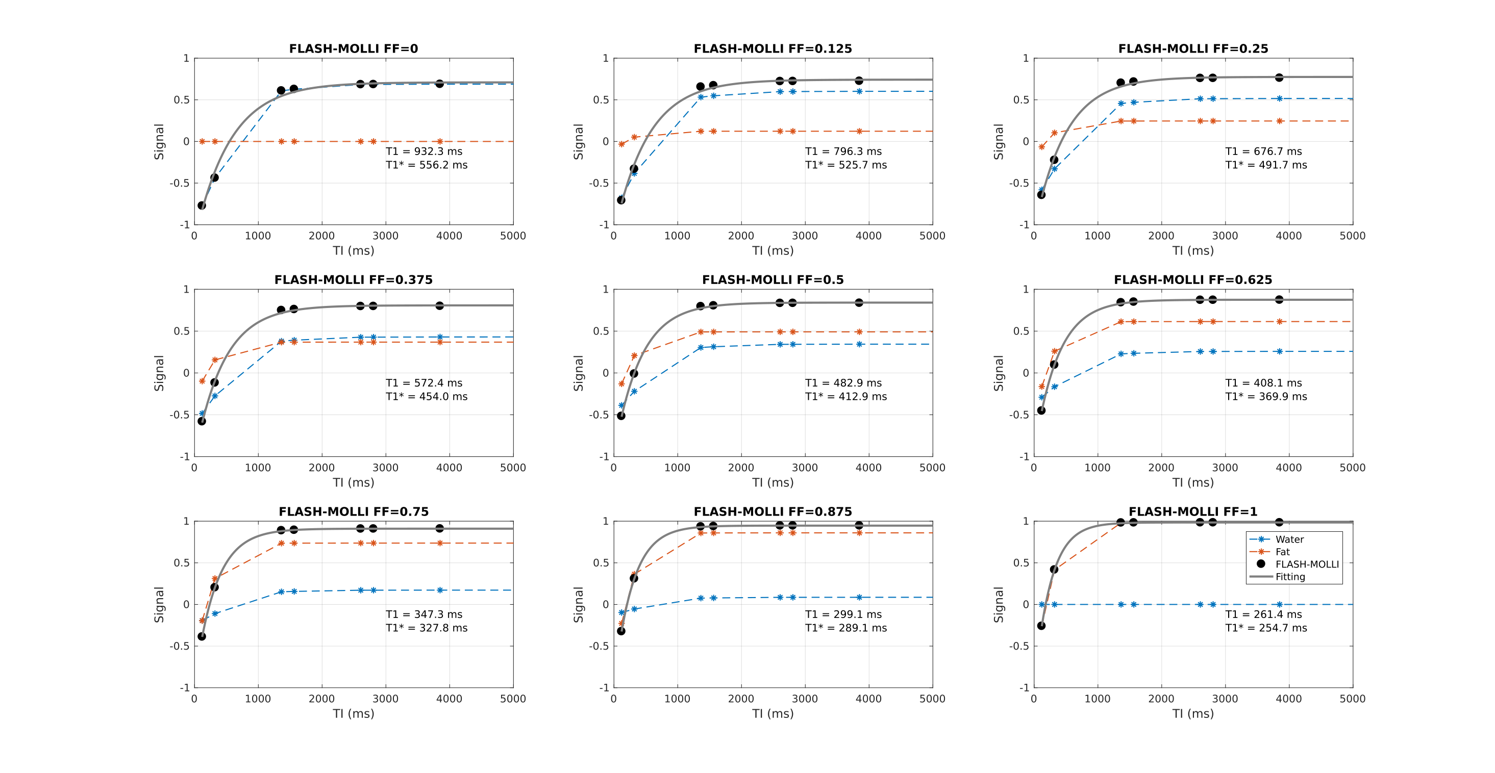
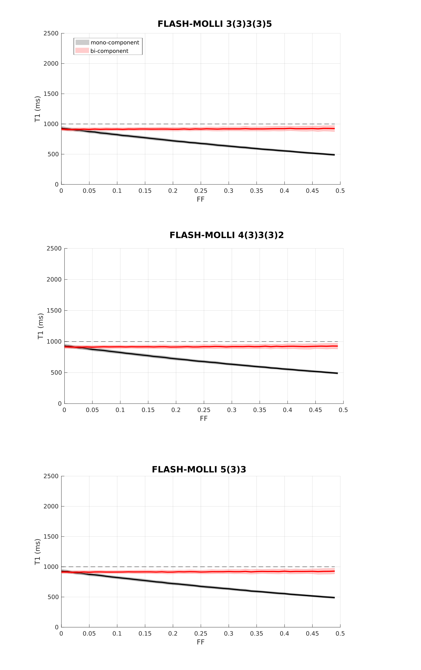
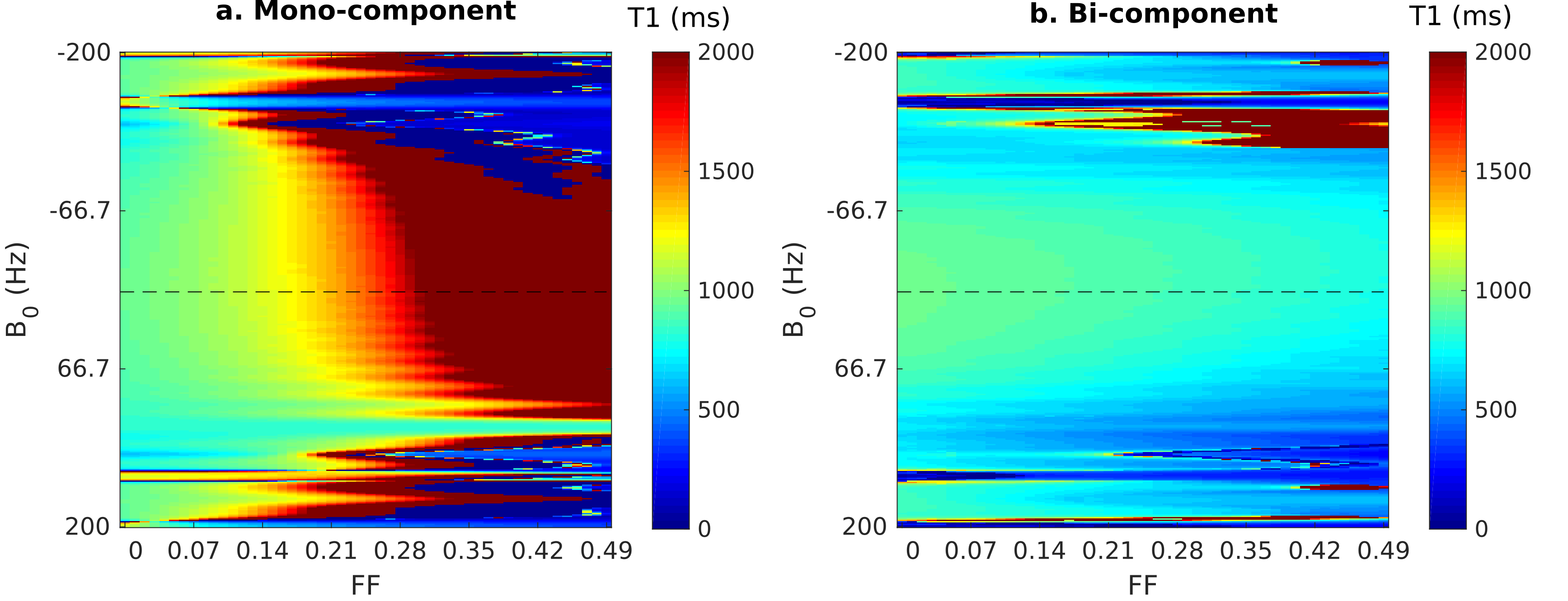
Figure 1 shows the signal evolution for FLASH-MOLLI at different fat fractions. The estimated T_1w with mono-component 3-parameter fitting shows a similar behaviour to that presented by bSSFP-MOLLI when water and fat are in phase (i.e. T_1w decrease with FF).³
The new bi-component model was able to correct the bSSFP-MOLLI behaviour for the tested FF range, with bias/precision error of 100/20ms, while improving robustness to ΔB₀ for higher FF values (Figure 4). However, the estimated T_1w still shows a FF dependency (Figure 2). With the FLASH readout, the results from the new model become stable, presenting bias/precision errors of 67/20ms for the FF range tested (Figure 3).

Discussion

bSSFP is a widespread readout method applied in cardiac MRI due to its high SNR. Nevertheless, it is very sensitive to ΔB₀, especially at high field strengths (i.e. 3T). This is particularly problematic in the presence of fat PVE. In contrast, the FLASH readout is known for its robustness to ΔB₀, but that comes at a cost of low SNR. The ΔB₀ robustness also explains why FLASH is less sensitive to fat infiltration than bSSFP, even with the standard mono-component 3-parameter fitting (Figure 1). Although bSSFP should enable a higher SNR which could improve precision, T_1w values could be off by 50% for FF=0.20 when using the mono-component model, which could lead to an erroneous diagnosis.⁹
The new bi-component model improved the accuracy of T_1w estimates for both readouts, and presents the advantage of estimating T_1w directly. The improvement for bSSFP-MOLLI shows that is possible to reduce bias for the sequences already available in clinical settings. Additionally, combining this method with FLASH-MOLLI has the potential to increase accuracy for FF by up to 50 %. Finally, this model would be readily applicable to new acquisition sequences recently proposed for T₁ estimation which already include Dixon measurements.¹⁰

Conclusion

The bSSFP-MOLLI sequence is widely available in the clinic but it is known to be very sensitive to fat signal contamination. To account for its impact, clinically available methods such as Dixon measurements could be used for separately measure FF and this information used to estimate accurate T_1W values with the proposed post-processing bi-component model fitting. This work shows that further improvements are also possible by using the new model in combination with a FLASH readout due to its robustness to ΔB₀. Further investigations are underway to evaluate these results in vivo.

Acknowledgements

Portuguese Foundation for Science and Technology (FCT - IF/00364/2013, UID/EEA/50009/2019, SFRH/BD/120006/2016), and POR Lisboa 2020 (LISBOA-01-0145-FEDER-029686).