3768
Compressed sensing applied to 1 mm isotropic multi-parametric imaging with 3D-QALAS: A phantom, volunteer, and patient study
Shohei Fujita1,2, Akifumi Hagiwara1, Naoyuki Takei3, Ken-Pin Hwang4, Issei Fukunaga1, Shimpei Kato1,2, Masaaki Hori5, Ryusuke Irie1,2, Christina Andica1, Toshiaki Akashi1, Koji Kamagata1, Ukihide Tateishi6, Osamu Abe2, and Shigeki Aoki1
1Department of Radiology, Juntendo University, Tokyo, Japan, 2Department of Radiology, The University of Tokyo, Tokyo, Japan, 3MR Applications and Workflow, GE Healthcare, Tokyo, Japan, 4Department of Radiology, MD Anderson Cancer Center, Houston, TX, United States, 5Department of Radiology, Toho University Omori Medical Center, Tokyo, Japan, 6Department of Radiology, Tokyo Medical and Dental University, Tokyo, Japan
1Department of Radiology, Juntendo University, Tokyo, Japan, 2Department of Radiology, The University of Tokyo, Tokyo, Japan, 3MR Applications and Workflow, GE Healthcare, Tokyo, Japan, 4Department of Radiology, MD Anderson Cancer Center, Houston, TX, United States, 5Department of Radiology, Toho University Omori Medical Center, Tokyo, Japan, 6Department of Radiology, Tokyo Medical and Dental University, Tokyo, Japan
Synopsis
Simultaneous relaxometry of T1, T2, and proton density by 3D-QALAS still requires relatively lengthy acquisition times and further acceleration is desired in clinical practice. Here, we applied compressed sensing combined with parallel imaging to 3D-QALAS to accelerate scan time. Quantitative values and tissue segmentation performance were compared with and without acceleration in phantom, healthy volunteers, and patients. With accelerated 3D-QALAS acquisition, whole brain 1 mm isotropic volume data with multiple parametric maps and co-registered tissue segmentation maps were obtained in less than 6 minutes, with comparable quality to 3D-QALAS without acceleration.
Introduction
Recent developments have enabled simultaneous quantitative T1, T2, and proton density (PD) mapping with a 3D acquisition. One such technique is 3D-quantification using an interleaved Look–Locker acquisition sequence with a T2 preparation pulse (3D-QALAS) sequence, which has recently been applied to the brain1 and has demonstrated high repeatability and reproducibility in vivo and in vitro.2 However, when unaccelerated, 3D-QALAS requires acquisition times that are relatively long for daily clinical use. Here, we propose the application of compressed sensing to 3D-QALAS sequence to enable whole brain 1 mm isotropic T1, T2, and PD quantification within 6 minutes.Methods
We implemented an acceleration technique that combined compressed sensing (CS) and data driven parallel imaging3,4 to 3D-QALAS. To evaluate the effects of CS acceleration on quantitative mapping and tissue segmentation, we acquired 3D-QALAS with and without CS for each subject. The CS acceleration factor was set to 1.9, based on a preliminary phantom study. The 3D-QALAS imaging parameters were all identical, except for the CS acceleration factor. The 3D-QALAS sequence imaging parameters were as follows: spatial resolution 1 × 1 × 1 mm, FOV = 25.6 × 20.5 × 14.6 cm, matrix = 256 × 205 × 146, TR/TE = 8.6/3.5 ms, bandwidth = 25 kHz, FA = 5 degrees. The scan times were 11:11 and 5:56 without and with CS, respectively. All subjects were scanned on a 3 T scanner (Discovery 750w, GE Healthcare, Waukesha, WI), with a 32-channel head coil.A standardized NIST/ISMRM phantom5 was scanned 10 times on different days, over a one-month period. The phantom was positioned 30 minutes prior to the scan to minimize effects of motion on the measurements. The original 3D QALAS sequence images were processed using a SyMRI software prototype (version 19Q3) to generate T1, T2, and PD maps. A spherical VOI was manually placed at the center of each sphere, on the T1, T2, and PD maps, and the respective mean values were recorded.
In vivo images of ten healthy volunteers were acquired in a study approved by the local institutional review board, with written informed consent obtained from all study participants. The T1, T2, and PD maps that were derived from 3D-QALAS with and without CS were compared based on semi-automated VOI analyses.6 For both datasets, tissue fraction maps and tissue volumes were calculated using SyMRI software.7 Ten patients with multiple sclerosis were also included in the study. A neuroradiologist identified plaques that were larger than 5 mm in diameter using all possible images. A spherical VOI was placed on each plaque and contralateral normal-appearing white matter (NAWM) to measure the mean T1, T2, and PD.
Simple linear regression analyses were performed for each metric obtained from the datasets with and without CS. A Bland-Altman analysis was performed to assess the agreement and biases between the T1, T2, and PD values that were obtained from 3D-QALAS with and without CS.
Results
Phantom StudyIn the phantom study, the T1, T2, and PD values that were measured with CS all showed strong linear correlations (R2 = 0.999 for T1; R2 = 0.993 for T2, R2 = 0.996 for PD) with the values measured without CS. The linear fits had slopes of 0.99 for the T1 values, 0.90 for T2, and 1.0 for PD, and the intercepts were 8.3 ms for T1, 15.2 ms for T2, and -0.1% for PD. The mean biases for T1, T2, and PD were -3.3 ms, 9.6 ms, and -0.3%, respectively. The 95% agreement limits for T1, T2, and PD ranged from -30.0 ms to 23.5 ms, -114.5 ms to 133 ms, and -2.5% to 1.9%, respectively.
Volunteer study
Figure 1 shows representative T1, T2, and PD maps and tissue fraction maps of the brain obtained from a healthy volunteer using 3D-QALAS with and without CS. Bland-Altman plots that show the agreement between with and without CS of the T1, T2, and PD values in different brain regions are shown in Figure 2. Figure 3 shows the agreement of the tissue fraction volumes that were calculated from 3D-QALAS with and without CS.
Patient study
Figure 4 shows a representative VOI placed on an MS plaque, overlaid on synthesized T1-weighted images. In total, 56 plaques were identified in 10 patients with MS. Figure 5 shows the biases of T1, T2, and PD values of the plaques, from the images obtained with and without CS.
Discussion
This study assessed the quantitative values and tissue segmentation performance of 3D-QALAS with and without CS acceleration. The relaxometry parameters and tissue volumes that were obtained with CS showed high agreement with those without CS. The rapid acquisition of relaxometry parameters in 6 minutes is comparable to our routine 3D structural imaging protocol, which requires 4-5 minutes. This approach will enable parameter mapping for disease characterization and the synthesis of contrast-weighted images for clinical use in routine brain protocols. Further investigations that assess the quality of the contrast-weighted 3D-QALAS images are needed.Conclusion
Isotropic 1 mm multi-parametric imaging of the whole brain based on 3D-QALAS can be performed in under 6 minutes using CS, while maintaining tissue quantitative values and segmentation accuracy.Acknowledgements
This study was grated for the Budget for promotion of strategic international standardization given by the Ministry of Economy, Industry, and Trade (METI).References
- Ken-Pin Hwang et al. 3D isotropic multi-parameter mapping and synthetic imaging of the brain with 3D-QALAS: comparison with 2D MAGIC. Proc. Intl. Soc. Mag. Reson. Med. 26 (2018), 5627.
- Fujita et al. Three-dimensional high-resolution simultaneous quantitative mapping of T the whole brain with 3D-QALAS: An accuracy and repeatability study. Magnetic Resonance Imaging. 2019;63:235–243
- Takei et al. Accelerated Compressed Sensing 3D multi-parametric imaging Toward Isotropic1mm3 Imaging. Proc. Intl. Soc. Mag. Reson. Med. 28 (2019), 5759.
- King et al. Compressed sensing description: “A New Combination of Compressed Sensing and Data Driven Parallel Imaging”. Proc. Intl. Soc. Mag. Reson. Med. 18 (2010), 4881.
- Keenan et al. Multi-site, multi-vendor comparison of T1 measurement using ISMRM/NIST system phantom. Proc. Intl. Soc. Mag. Reson. Med. 24 (2016), 3290
- Hagiwara A et al. Linearity, bias, intrascanner repeatability, and interscanner reproducibility of quantitative multidynamic multiecho sequence for rapid simultaneous relaxometry at 3 T: a validation study with a standardized phantom and healthy controls. Invest Radiol 2019;54(1):39–47.
- West J et al. Novel whole brain segmentation and volume estimation using quantitative MRI. Eur Radiol. 2012;22:998–1007.
Figures
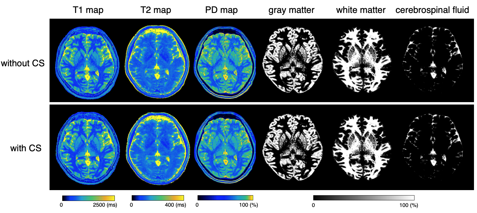
Figure 1. Representative quantification maps and tissue fraction maps of a healthy volunteer. Axial images of T1, T2, PD maps and segmentation results for gray matter, white matter, and cerebrospinal fluid. Minimal differences are seen between the maps that were obtained with and without CS. PD, proton density; CS, compressed sensing.
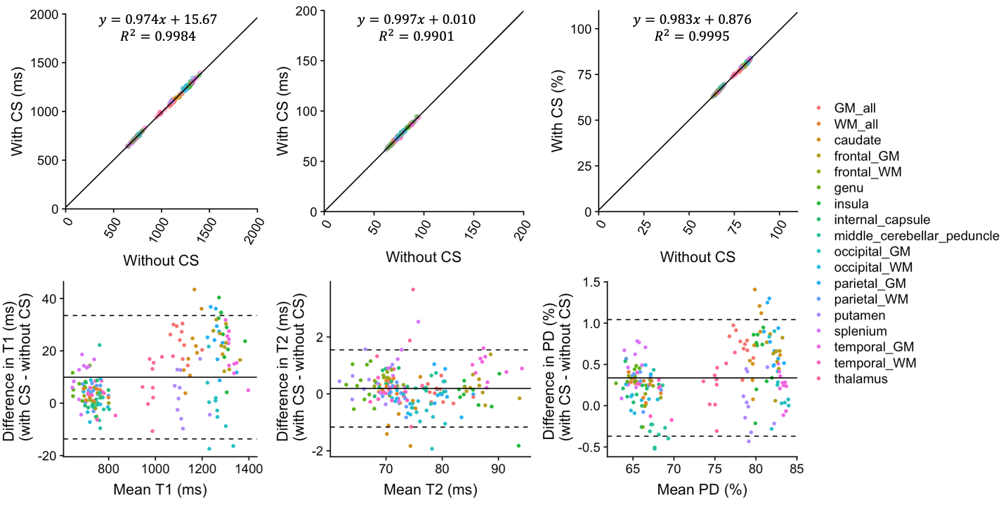
Figure 2. Scatterplots and Bland-Altman plots comparing T1, T2, and PD values of 16 brain regions that were calculated from 3D-QALAS with CS compared to those calculated without CS. Solid black lines in the scatterplots represent the linear regression fit, and the center solid lines in the Bland-Altman plots represent mean differences. The upper and lower dotted lines represent the agreement limit, which was defined as the mean difference ± 1.96 × SD of the difference between the values acquired with and without CS. SD, standard deviation.
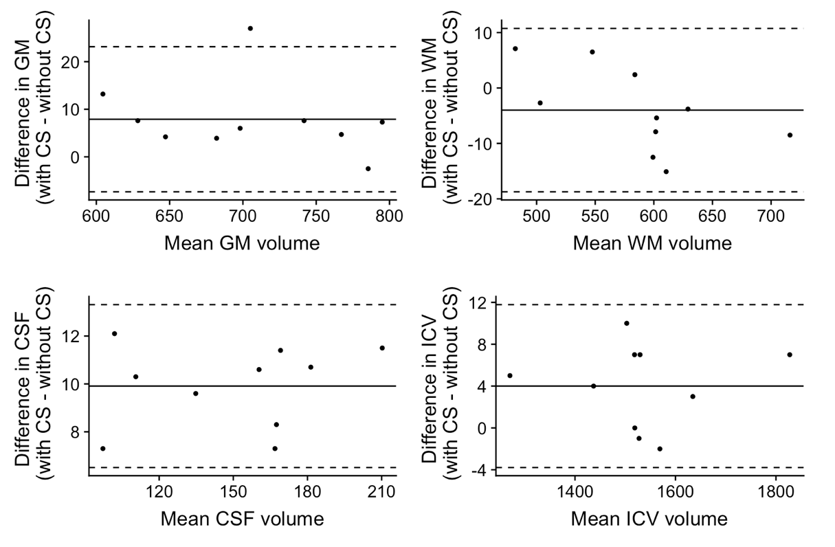
Figure 3. Bland-Altman plots comparing GM, WM, CSF, and ICV volumes of 10 volunteers, calculated from 3D-QALAS acquired with and without CS. The center solid lines represent mean differences, while the upper and lower dotted lines represent the limit of agreement, which is defined as the mean difference ± 1.96 × SD of the difference between the values acquired with and without CS. SD, standard deviation, GM, gray matter; WM, white matter; CSF, cerebrospinal fluid; ICV, intracranial volume.
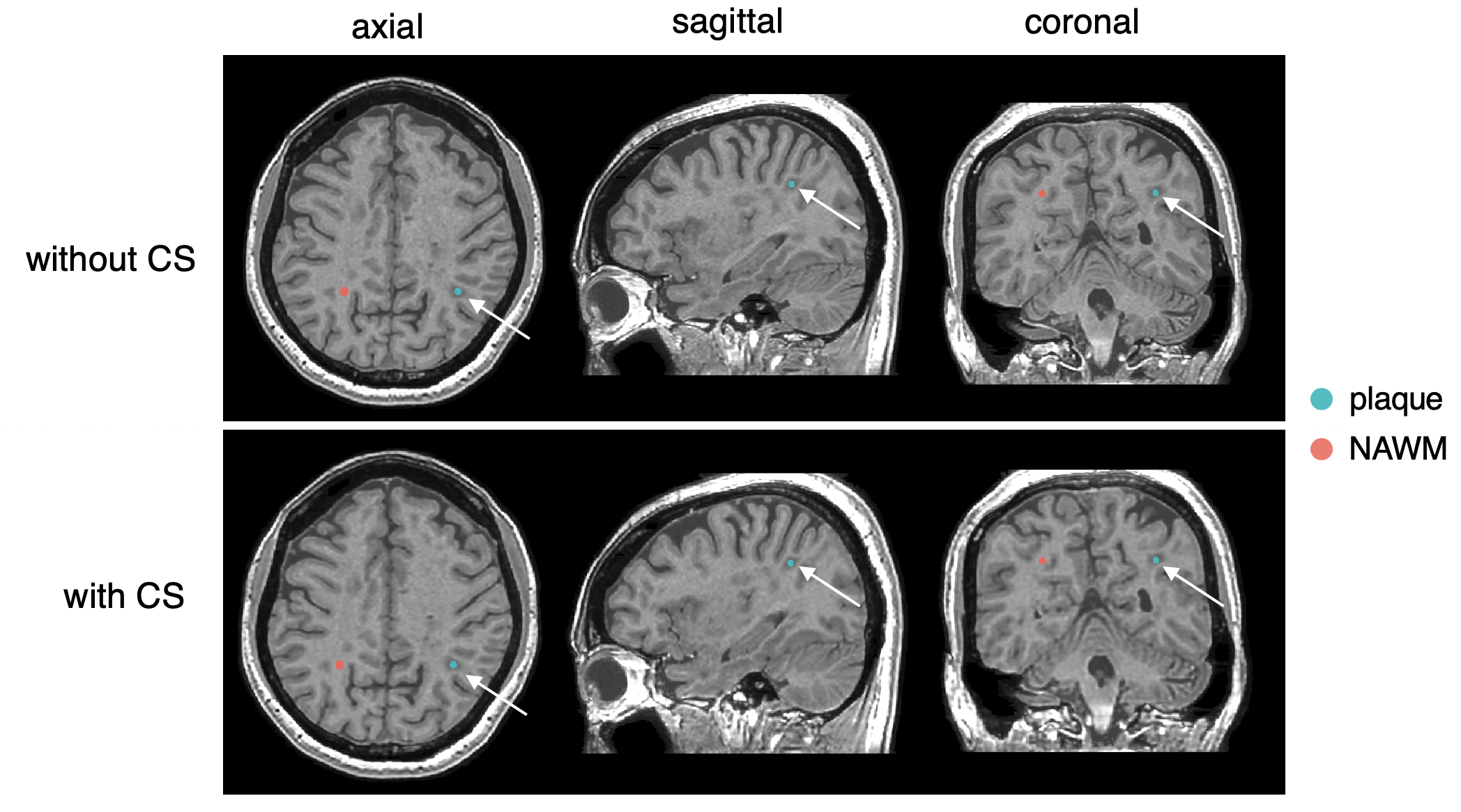
Figure 4. An example of spherical VOI placement in a patient with multiple sclerosis. A plaque (arrow) is shown on synthetic T1-weighted images; a spherical VOI was placed in the center of the plaque (blue). The VOI was copied and pasted on the contralateral NAWM (red). VOI; volume of interest; NAWM, normal-appearing white matter.
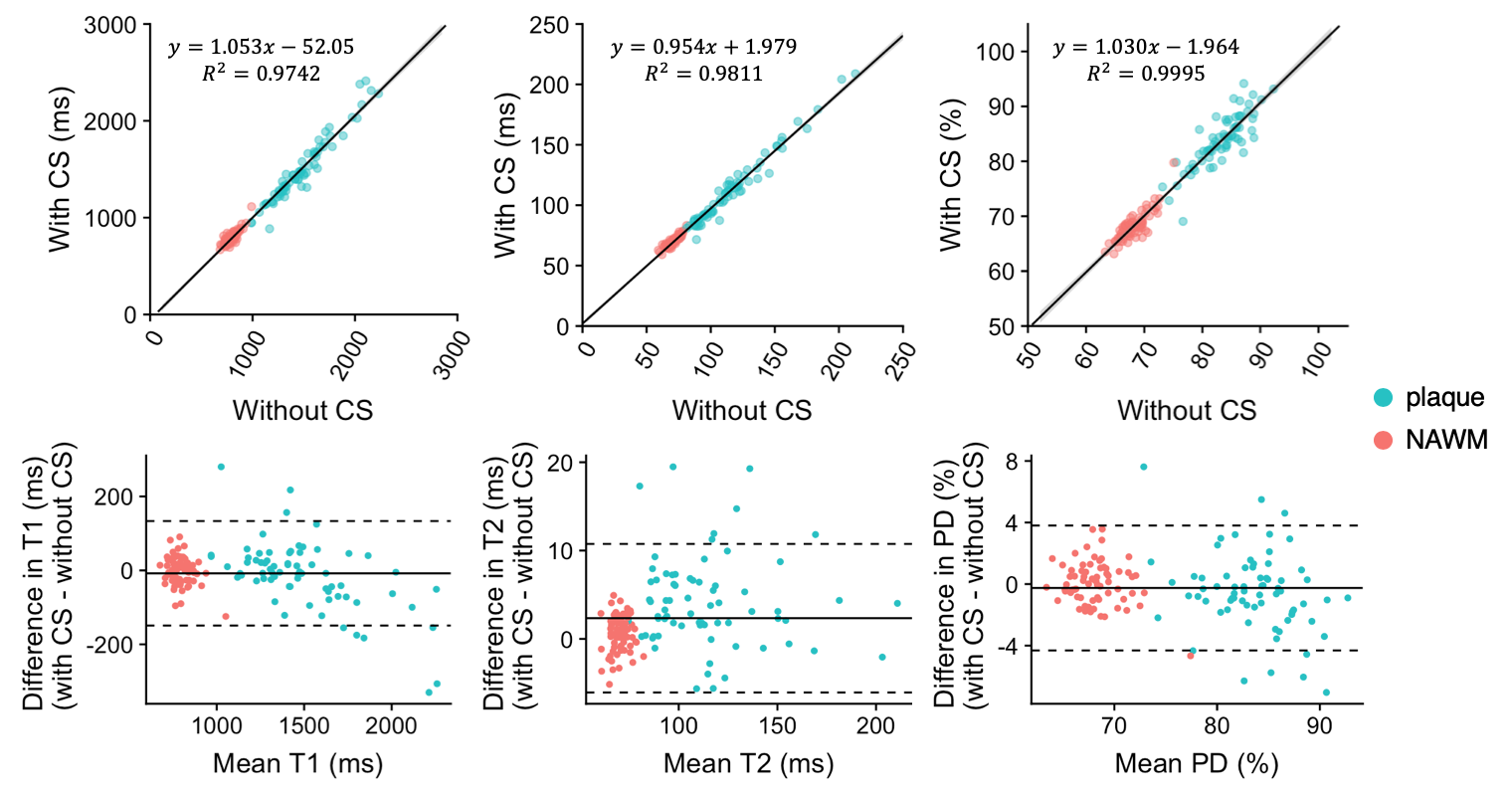
Figure 5. Scatterplots and Bland-Altman plots comparing T1, T2, and PD values of plaques and NAWM calculated from 3D-QALAS acquired with and without CS. The solid black lines in the scatterplots represent the linear regression fit, and the center solid lines of the Bland-Altman plots represent mean differences. The dotted lines represent the agreement limit, which was defined as the mean difference ± 1.96 × SD of the difference between the measurements with and without CS. NAWM, normal-appearing white matter.