Introduction

Magnetic Resonance Fingerprinting (MRF) is a novel imaging technique capable of simultaneous mapping of multiple tissue and system properties¹. MRF data is typically acquired with fast sampling of highly undersampled k-space with a temporally variable FA/TR. The reconstructed MRF signal evolutions are assumed to be encoded by the underlying tissue properties which are then obtained with dictionary matching. The dictionary is simulated considering the possible tissue and system property ranges (field inhomogeneities, slice profile, etc.). Because of this, the accuracy of MRF maps depends on the exact knowledge of system properties throughout the acquisition. Recent experiments revealed ~4-5 Hz/min scanner frequency drifts during continuous 2D MRF acquisitions due to the eddy currents from fast switching gradients. If not accounted for, any discrepancy between the expected and the real on-resonance frequency might cause problems in the dictionary matching stage. Here we incorporate experimental measurements of frequency drifts into dictionary generation and suggest a novel MRF reconstruction framework for 3D. Improved image quality is shown when these drifts are taken into account.

Methods

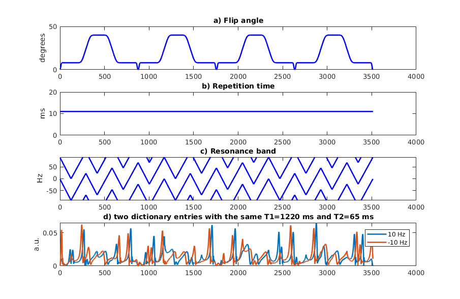
Recently, MRF with quadratic RF phase² (MRFqRF) was introduced to map off-resonance and T2*, in addition to T1 and T2. Since MRFqRF is particularly sensitive to frequency drifts with artifacts as blurring in T1 maps and overestimation of Γ, it is a good candidate to test our hypothesis.
2D MRFqRF brain data³: 256x256 matrix size, 1.2x1.2 mm² resolution, 5 mm slice thickness, 3516 time points (t_p). 3D MRFqRF brain data⁴: 24 partitions (N_p), same acquisition parameters as in 2D (Figure 1) but with 3D excitation and phase encoding in z-direction with no acceleration. Also for reference, 3D FISP MRF data (matching MRFqRF FOV) were also acquired. Informed consent with IRB approval was obtained prior to the data acquisition.
For frequency drift estimation, we acquired 10 consecutive 2D MRFqRF scans and calculated the mean off-resonance change per TR over an ROI. Then, for frequency drift compensated MRFqRF dictionary, every entry was updated every TR with an increment of the resulting mean frequency drift of 0.0013 Hz/TR within the Bloch simulations. Dictionary and the data were compressed with randomized SVD⁵ (rSVD) prior to the reconstruction. The dictionary was also undersampled in the tissue property dimension. Quadratic interpolation⁶ recovers the high resolution in the tissue property dimension. The same 2D MRFqRF data were reconstructed with the generic and frequency drift compensated MRF dictionary.
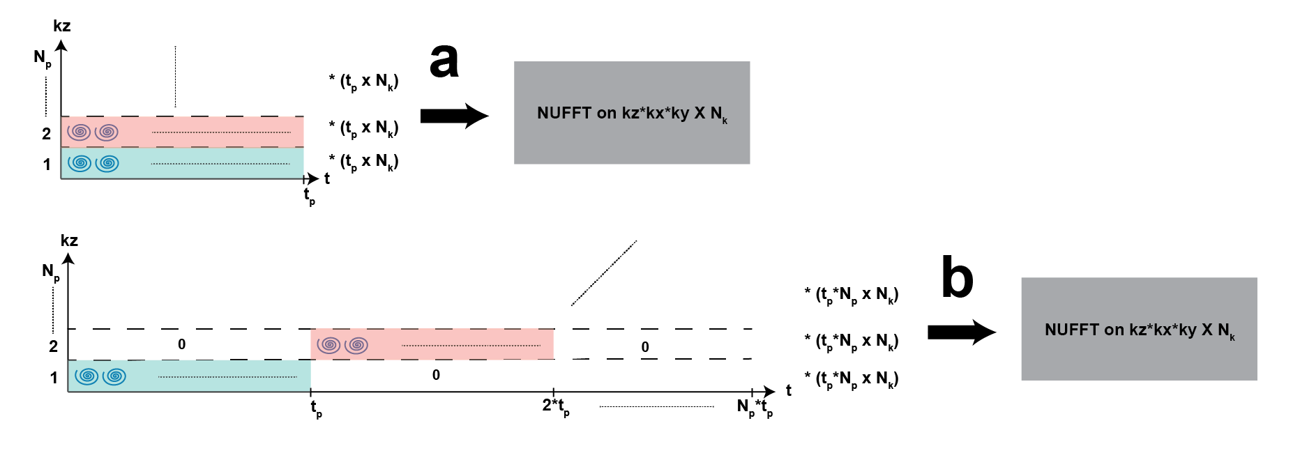
During generic 3D MRF reconstruction each k-space partition is compressed to Nk rank with the compression matrix calculated from rSVD of the standard dictionary (Figure 2a). Then, Nk fully sampled k-space data go through non-uniform FFT and the resulting Nk images get matched to the compressed dictionary. However, in the case of frequency drift, each partition will have a frequency offset of an integer multiple of t_p*0.0013 Hz compared to the very first time point in the acquisition. In this case, the compression matrix, even though it’s calculated from the frequency drift compensated 2D dictionary, would only apply to the first partition and not the others. To overcome this problem, we suggest a new framework for 3D MRF reconstruction (Figure2b) where we calculate one SVD that can compress all partitions than might have slightly different signal evolutions due to the drift. The same 3D MRFqRF data were reconstructed with the generic and frequency drift corrected dictionary for comparison.

Results

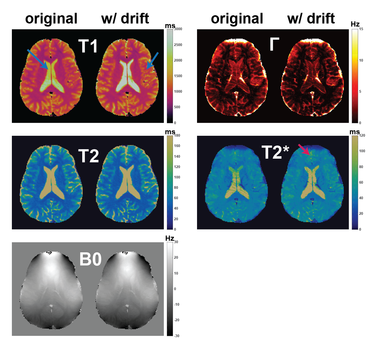
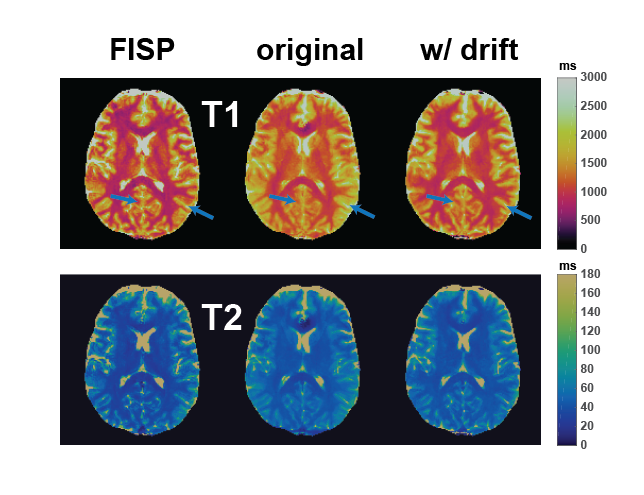
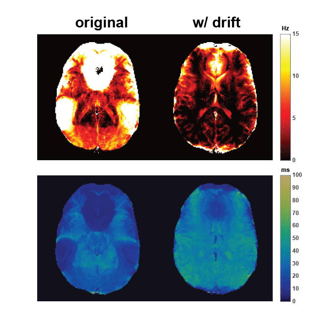
2D results are shown in Figure 3. Frequency drift correction mainly improves the underestimation of T1 over the whole brain but most dramatically in ventricles. Γ values are overall decreased and T2* contrast gets sharper.
Improvement in 3D T1 maps is noteworthy (Figure 4). Compared to FISP, there’s significant blurring in T1 maps with standard reconstruction which is practically corrected with frequency drift compensation. 3D Γ maps might be improved the most (Figure 5) since with frequency drift it does not have to explain all the frequencies that existed in the voxel throughout the acquisition. 3D T2* maps have similar contrast to 2D T2* maps.

Discussion and Conclusions

Here, upon the observation of scanner frequency drifts during dynamic MRFqRF scans and its possible effects, two potential retrospective correction schemes are suggested. For 2D MRF, the dictionary can be updated with manual increments of measured frequency drifts to compensate for unexpected differences between the acquired data and the dictionary. For 3D MRF, a new reconstruction framework is introduced. The results show significant improvements especially for T1 and T2* maps.
The frequency drift is specific to our system and sequence and could be different on other scanners. Here this value was manually hardcoded into the dictionary but one can also consider making a frequency drift dimension in the dictionary (assuming its time evolution, i.e. linear) and obtain the frequency drift with dictionary matching.
3D reconstruction framework introduced here opens the door to different and optimized sequence parameters for each partition. Thus, MRF optimization problem may have more degrees of freedom and not be limited to number of time points per partition.
In conclusion, it is necessary to compensate for the frequency drift in MRF, especially for bSSFP based MRF sequences, to obtain accurate quantitative maps and a simple retrospective framework achieving that was described.

Acknowledgements

This work is supported by Siemens Healthcare.