3689
Optimal Flip Angle Formula for SWIFT and CEA (Concurrent Excitation and Acquisition) MRI1Dept. of Radiology, Medical Physics, Medical Center – University of Freiburg, Freiburg, Germany, 2Center for Magnetic Resonance Research and Department of Radiology, University of Minnesota, Minneapolis, MN, United States, 3German Consortium for Translational Cancer Research Partner Site Freiburg, German Cancer Research Center (DKFZ), Heidelberg, Germany
Synopsis
MR imaging of tissue components with extremely fast transverse relaxation times require advanced MRI techniques such as continuous SWIFT (cSWIFT), Concurrent Excitation and Acquisition (CEA), and full duplex MRI. Frequency modulated pulses are used in these methods. A steady-state signal model with transverse relaxation term was formulated and solved for an arbitrary frequency and phase modulated RF pulse. An accurate expression for the optimal flip angle was derived. The performance of the new formulation was verified by a home-made Bloch equation simulator for T2 values between 10µs and 100ms.
Introduction
For MR imaging of tissues with extremely fast T2-decays, such as myelin and cortical bone(1), sweep imaging with Fourier transformation (SWIFT) method has been developed (2) which was followed by concurrent RF excitation and signal acquisition (CEA) methods(3–7) that offer a 100% receiver duty cycle. In SWIFT and CEA, frequency-modulated (FM) hyperbolic secant (HSn) pulses are used for excitation. FM methods can offer a broader band excitation and acquisition than hard pulse methods(8,9), as the bandwidth is limited only by the frequency-sweep range in the former case and the peak RF power in the latter.To adjust the contrast and to maximize SNR in SWIFT and CEA, the steady‑state (SS) behavior of the sequence must be analyzed. For HS1 pulses an analytical solution to the Bloch equations was developed to optimize sequence timing and FM parameters; however, this solution does not account for T2 relaxation(10). In addition, the equations for the maximum MR signal for hard pulse methods are not applicable to CEA. Current simplified methods (SM)(11,12) first approximate the FM pulse by a hard pulse of the same flip angle and pulse duration and then use the Ernst equation to calculate the SS signal. CEA, however, requires a more accurate signal model which includes the T2-decay. In this study, we formulated the SS magnetization during CEA with HSn pulses and verified the accuracy for different T2 values with a Bloch simulation.
Methods
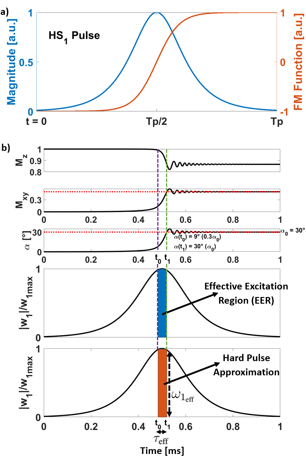
A continuous FM RF pulse (as is used in a CEA sequence) was represented as a series of short rectangular pulses of duration δ, and analytical solutions to the Bloch equations (13) were calculated for each δ pulse.FM pulses in CEA sweep through the resonance at t = Tp/2 (Tp : pulse length). For an accurate flip angle estimation we define an effective excitation time ($$$\tau_\text{eff}$$$), which is empirically set to the time between a flip angle of 0.3α0 and α0, where α0 is the desired flip angle. HS1 pulses can be represented by a hard pulse using the $$$\tau_\text{eff}$$$ definition as shown in Fig. 1 (effective pulse approximation, EPA). We define the effective RF energy, which excites the spins during $$$\tau_\text{eff}$$$: $$\text{En}_\text{eff} = \int_{t_0}^{t_1} |w_1(t)|^2 dt,$$ where ω1 is the complex RF pulse and, t0 and t1 are the start and end points of the Effective Excitation Region (EER), respectively. Then, we calculated the effective RF amplitude as: $$$\omega_{1_\text{eff}} = \sqrt{\frac{\text{En}_\text{eff}}{\tau_{\text{eff}}}}$$$.
In this study, for comparison we used the modified Ernst equation (14) which takes T2-decay into account: $$E_1 = e^{-\frac{\text{TR}}{T_1}}$$ $$E_{2_\text{eff}} = e^{-\frac{\tau_{\text{eff}}}{2T_2}}$$ $$a_{\text{eff}} = \sqrt{\omega_{1_\text{eff}} ^2-\frac{1}{(2 T_2)^2}}$$ $$M_{xy}^{SS} = M_0 \frac{(1-E_1)\omega_{1_\text{eff}} E_{2_\text{eff}} sin(a_{\text{eff}}\tau_{\text{eff}})}{a_{\text{eff}}\left\lbrace1-E_1 E_{2_\text{eff}}\left[\cos(a_{\text{eff}}\tau_{\text{eff}})+\frac{1}{2 T_2a_{\text{eff}}}\sin(a_{\text{eff}}\tau_{\text{eff}})\right]\right\rbrace}$$
To validate the proposed method, for a myelin (T1=200 ms, T2=114 µs) the SNR improvement of the signal was simulated using the parameters of Tp=4 ms and TR=8 ms.
Results
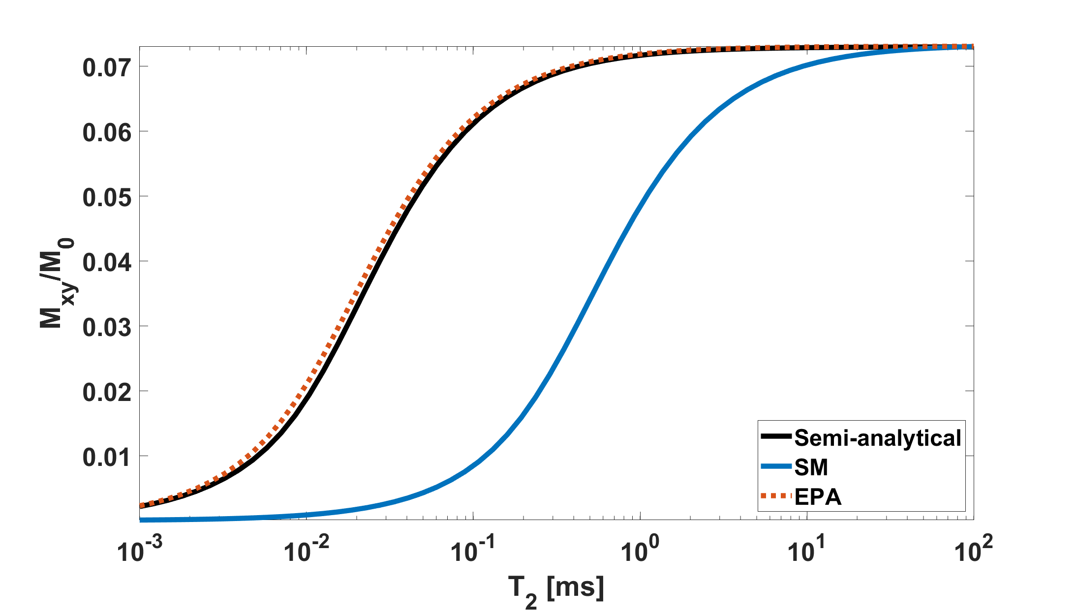
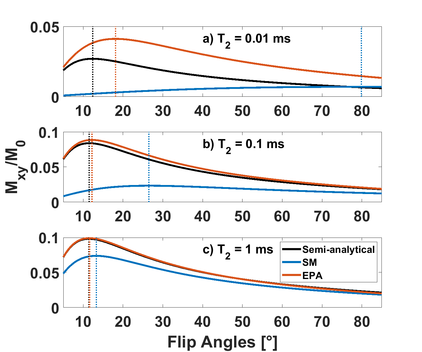
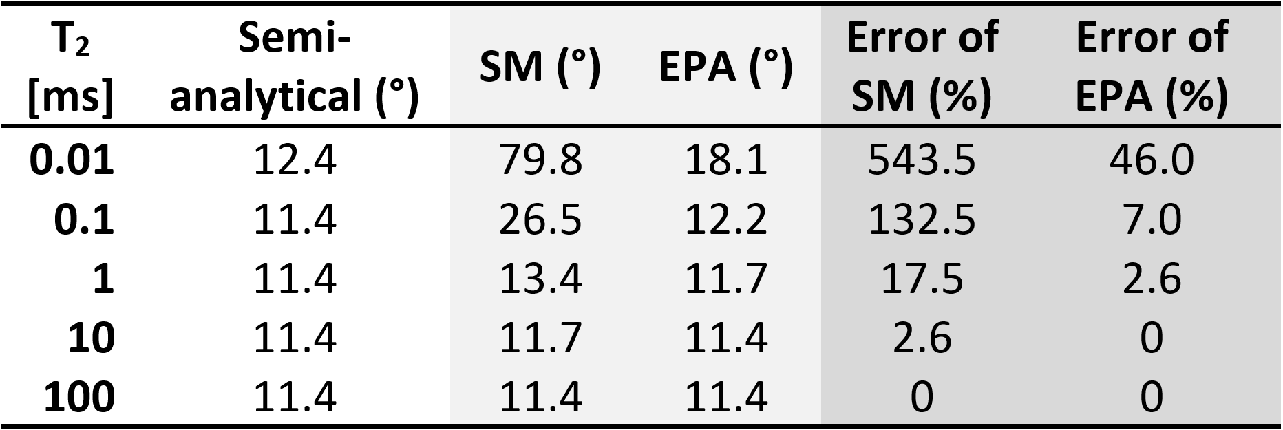
In Figure 2, the simulation results of the SS transverse magnetization excited by an HS1 pulse of α=5° with SM and EPA are shown. EPA has a superior accuracy for all T2 values: the error of EPA is smaller than 2% for T2 values higher than 70 µs, whereas SM deviates by more than 50% when T2 is less than 0.5 ms.In Figure 3, the SS transverse magnetization Mxy is shown with respect to the flip angle. For sub-ms T2 values, the optimal flip angles predicted by SM deviate significantly from the true optimum (vertical lines in Figure 3) with errors of 132% / 543% for T2=100 / 10 µs. The results of the Fig. 3 are summarized in Table 1.
An optimal α = 16.5° was found in the simulations for myelin, whereas the optimal calculated values were 66.2° and 19.5° for SM and EPA, respectively. With these values, the SS signal of myelin was simulated and a 2.34-fold higher SNR was found for EPA compared to SM.
Discussion
The optimal flip angle expression introduced in this work can be used to maximize steady-state signal in CEA experiments. Compared to a Bloch simulation, this expression can be used to analytically predict the optimal flip angle, so that protocol optimization for MRI and MRS is easily possible for tissue with ultra-short T2.For extreme T2 < 10µs, the error range of EPA also increases. However, a large variety of human tissue has T2 larger than 10µs. The validity of our tool needs to be tested for a more general class of FM RF pulses.
Acknowledgements
No acknowledgement found.References
1. Weiger M, Pruessmann KP. Short-T2 MRI: Principles and recent advances. Prog. Nucl. Magn. Reson. Spectrosc. 2019 doi: 10.1016/j.pnmrs.2019.07.001.
2. Idiyatullin D, Corum C, Park JY, Garwood M. Fast and quiet MRI using a swept radiofrequency. J. Magn. Reson. 2006;181:342–349 doi: 10.1016/j.jmr.2006.05.014.
3. Idiyatullin D, Suddarth S, Corum CA, Adriany G, Garwood M. Continuous SWIFT. J. Magn. Reson. 2012;220:26–31 doi: 10.1016/j.jmr.2012.04.016.
4. Özen AC, Bock M, Atalar E. Active decoupling of RF coils using a transmit array system. Magn. Reson. Mater. Physics, Biol. Med. 2015;28:565–576 doi: 10.1007/s10334-015-0497-0.
5. Salim M, Özen AC, Bock M, Atalar E. DETECTION OF MR SIGNAL DURING RF EXCITATION USING FULL DUPLEX RADIO SYSTEM. In: International Society for Magnetic Resonance in Medicine. ; 2016.
6. Özen AC, Atalar E, Korvink JG, Bock M. In vivo MRI with Concurrent Excitation and Acquisition using Automated Active Analog Cancellation. Sci. Rep. 2018;8 doi: 10.1038/s41598-018-28894-w.
7. Sohn S-M, Vaughan JT, Lagore RL, Garwood M, Idiyatullin D. In Vivo MR Imaging with Simultaneous RF Transmission and Reception. Magn Reson Med. 2016;76:1932–1938 doi: 10.1002/mrm.26464.
8. Weiger M, Pruessmann KP, Hennel F. MRI with zero echo time: Hard versus sweep pulse excitation. Magn. Reson. Med. 2011;66:379–389 doi: 10.1002/mrm.22799.
9. Garwood M. MRI of fast-relaxing spins. J. Magn. Reson. 2013;229:49–54 doi: 10.1016/j.jmr.2013.01.011.
10. Zhang J, Garwood M, Park JY. Full analytical solution of the bloch equation when using a hyperbolic-secant driving function. Magn. Reson. Med. 2017;77:1630–1638 doi: 10.1002/mrm.26252.
11. Tong G, Geethanath S, Vaughan JT. On the signal strength of Simultaneous Transmission and Reception (STAR) acquisition: EPG simulation and analysis. In: Proc. Intl. Soc. Mag. Reson. Med. ; 2019.
12. O’Connell RD. Determining Optimum Imaging Parameters for SWIFT : Application to Superparamagnetic Iron Oxides and Magnetized Objects. University of Minnesota; 2011.
13. Morris GA, Chilvers PB. General Analytical Solutions of the Bloch Equations. J. Magn. Reson. Ser. A 1994;107:236–238 doi: 10.1006/jmra.1994.1074.
14. Carl M, Bydder M, Du J, Takahashi A, Han E. Optimization of RF Excitation to Maximize Signal and T2 Contrast of Tissues With Rapid Transverse Relaxation. 2010;490:481–490 doi: 10.1002/mrm.22433.
Figures