3676
Perceptual Noise-Estimation based Method for MRI denoising with deep learning
Xiaorui Xu1, Siyue Li1, Shutian Zhao1, Chun Ki Franklin Au1, and Weitian Chen1
1CUHK lab of AI in radiology (CLAIR), Department of Imaging and Interventional Radiology, The Chinese University of Hong Kong, Hong Kong, Hong Kong
1CUHK lab of AI in radiology (CLAIR), Department of Imaging and Interventional Radiology, The Chinese University of Hong Kong, Hong Kong, Hong Kong
Synopsis
Most of the methods in MRI denoising derive denoised images from corrupted images directly. DnCNN is a network that is used to remove Gaussian noise from natural images. The noise distribution in MRI images are often non-Gaussian due to the latest development of reconstruction algorithm and MRI hardware. In this work, we investigated the case when the noise follows Racian distribution. We utilized the idea of DnCNN and combine it with a perceptual architecture to remove Rician noise of MRI images. We demonstrated this method can generate ideal clean images.
Introduction
Many MRI applications are hindered due to signal-to-noise ratio (SNR) limit in MRI. Thus, robust and reliable denoising technologies are highly desirable in MRI. Most of the denoising methods based on deep learning in MRI generate denosied images from noisy images directly. These methods may result in artifacts because it is not easy to learn the mapping relation between noisy images and clean images due to the complex anatomical structures. Besides, denoising of MRI images inevitably leads to smoothing of images and loss of certain details. DnCNN [1] was reported to have a good performance on removing Gaussian noise on natural images. In this work, based on DnCNN, we aim to estimate the noise of MRI images, and derive denoised MRI images with retained object structure and texture details.Methods
The basic idea of DnCNN [1] is to learn how to estimate noise from corrupted images. DnCNN (Figure 1) utilizes L2 loss function to minimize the error, but L2 loss has been proved to result in fuzzy results. Therefore, we use L1 loss to replace the previous L2 loss function in DnCNN and define this method as DnCNN_L1 (Figure 1). L2 loss and L1 loss only measure the pixel-wise error between two images, which lacks the capacity to generate images that meet human perceptual system. Hence, we choose feature extraction part of pre-trained vgg19 and concatenate it with the DnCNN. The generated noise image and real noise image can then be fed into the feature extraction part of vgg19 to generate fake noise feature and real noise feature which can be used to calculate perceptual loss. Perceptual loss can be formulated as Lperceptual = 1/(w * h) * ||VGG(G(x)) - VGG(y) ||2 , where G(x) and y represent generated noise image and real noise image, and w and h are the width and height of extracted feature maps. DnCNN, with L1 loss and L2 loss respectively, utilizes feature extraction architecture is denoted as DnCNN_L1_Perceptual and DnCNN_L2_perceptual (Figure 2). The clean T1-weighted images for training and testing were collected from a Philips Achieva 3.0T system (Philips Achieva, Philips Healthcare, Best, Netherlands). The corresponding corrupted T1-weighted images were synthesized by adding certain level of Rician noise. Afterwards, we derived related noise images for training by subtracting clean images from corrupted images. The size of the collected images is 720 * 720. Considering the memory of GPU, we split the images into patches with patch size 48 * 48 to input the network and increase the depth of the network into 24 for better receptive field. The metrics we used to quantitatively evaluate the performance are PSNR and SSIM, which can assess the fidelity and similarity between clean images and denoised images.Results and Discussion
Figure 3 compares the results from DnCNN, DnCNN_Perceptual, DnCNN_L1 and DnCNN_L1_Perceptual. Note DnCNN with L2 loss cannot estimate Rician noise accurately, compared with using L1 loss. Besides, DnCNN_Perceptual and DnCNN_L1_Perceptual outperform DnCNN and DnCNN_L1, which proves the effectiveness of perceptual loss. As is shown in the zoom-in region in Figure 3, DnCNN_L1_Perceptual derives the best denoised images and reserves the best texture details. Figure 4 illustrates the PSNR and SSIM of DnCNN, DnCNN_Perceptual, DnCNN_L1 and DnCNN_L1_Perceptual on the test T1-weighted dataset, which also demonstrates the advantages of using L1 loss and perceptual loss. Figure 5 compares the performance of DnCNN_L1_Perceptual, BM3D [2], and Non-Local Means (NLM) [3]. Note the DnCNN_L1_Perceptual achieved superior performance compared to these two classic denoising methonds in terms of visual effect and quantitative metrics.Conclusion
We demonstrated that DnCNN architecture combined with L1 loss and perceptual loss derived from vgg network achieves significant improvement in MRI denoising compared to DnCNN itself.Acknowledgements
This study is supported by a grant from the Innovation and Technology Commission of the Hong Kong SAR (Project MRP/001/18X), and a grant from the Research Grants Council of the Hong Kong SAR (Project SEG CUHK02).References
- K. Zhang, W. Zuo, Y. Chen, D. Meng and L. Zhang, "Beyond a Gaussian Denoiser: Residual Learning of Deep CNN for Image Denoising," in IEEE Transactions on Image Processing, vol. 26, no. 7, pp. 3142-3155, July 2017.
- K. Dabov, A. Foi, V. Katkovnik, and K. Egiazarian, "Image Denoising by Sparse 3D Transform-Domain Collaborative Filtering," IEEE Transactions on Image Processing, vol. 16, no. 8, August, 2007.
- R. Verma and R. Pandey, "Non local means algorithm with adaptive isotropic search window size for image denoising," 2015 Annual IEEE India Conference (INDICON), New Delhi, 2015, pp. 1-5. doi: 10.1109/INDICON.2015.7443193.
Figures
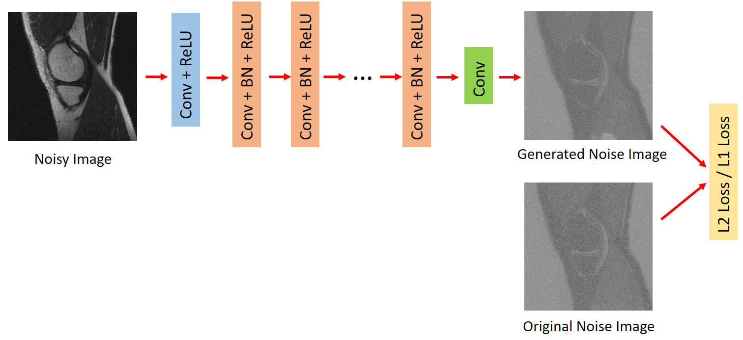
Figure 1: Architecture of DnCNN and DnCNN_L1. The original
DnCNN uses L2 loss. The proposed DnCNN_L1 uses L1 loss.
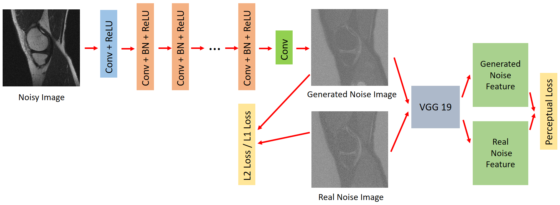
Figure 2: Architecture of DnCNN_Perceptual and DnCNN_L1_Perceptual.
DnCNN concatenated with the feature extraction part of vgg19 to calculate the
perceptual loss is DnCNN_Perceptual, and DnCNN_L1 with perceptual loss is called
DnCNN_L1_Perceptual.
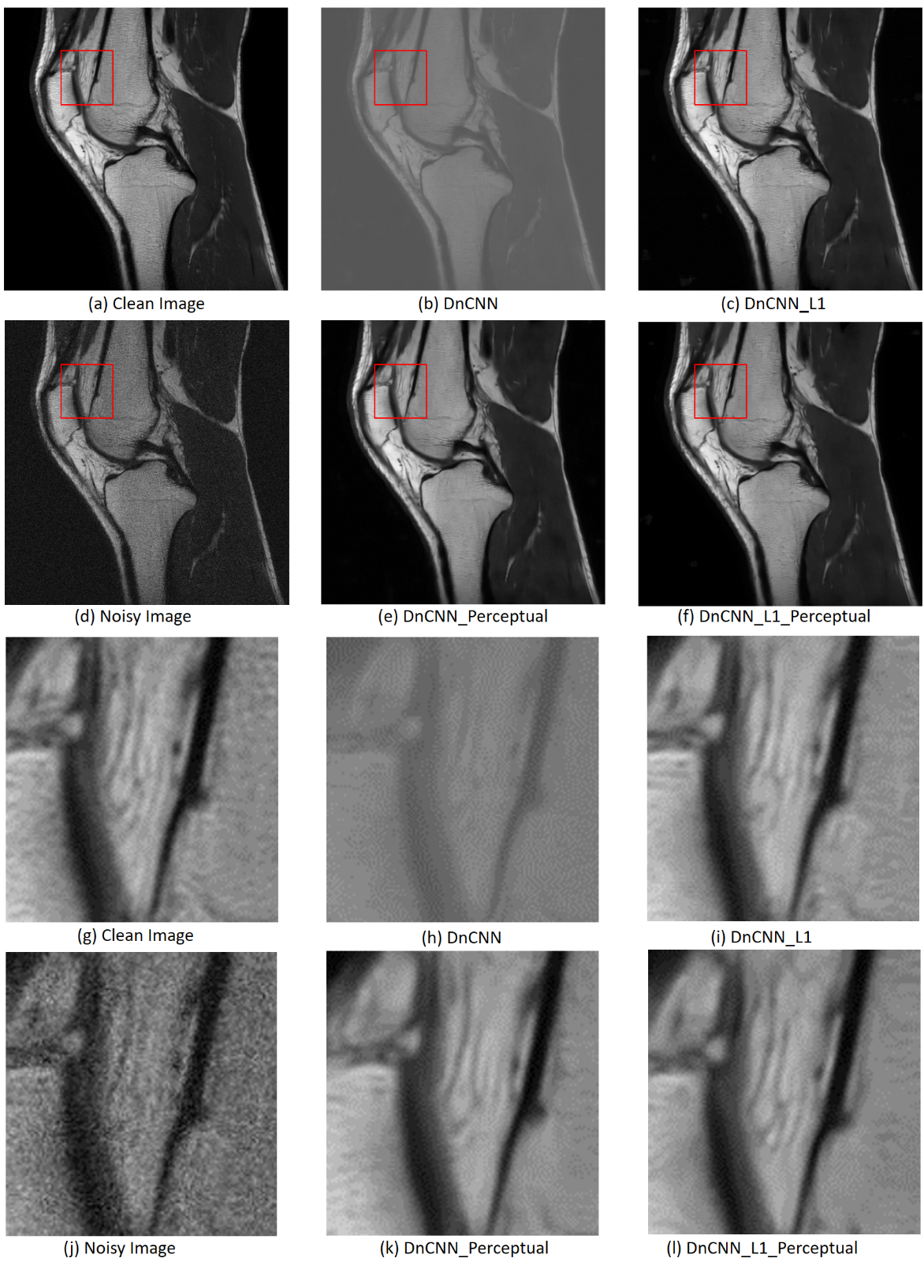
Figure 3: Visual Comparison between clean image, noisy image
and denoised images generated by DnCNN, DnCNN_Perceptual, DnCNN_L1 and
DnCNN_L1_Perceptual. (a) to (f) are the images with full FOV. (g) to (I) show
the zoom-in region. PSNR and SSIM of DnCNN, DnCNN_Perceptual, DnCNN_L1 and
DnCNN_L1_Perceptual concerning these images are (12.02db, 0.39), (33.29db, 0.75),
(31.41db, 0.77) and (33.77db, 0.84) respectively.
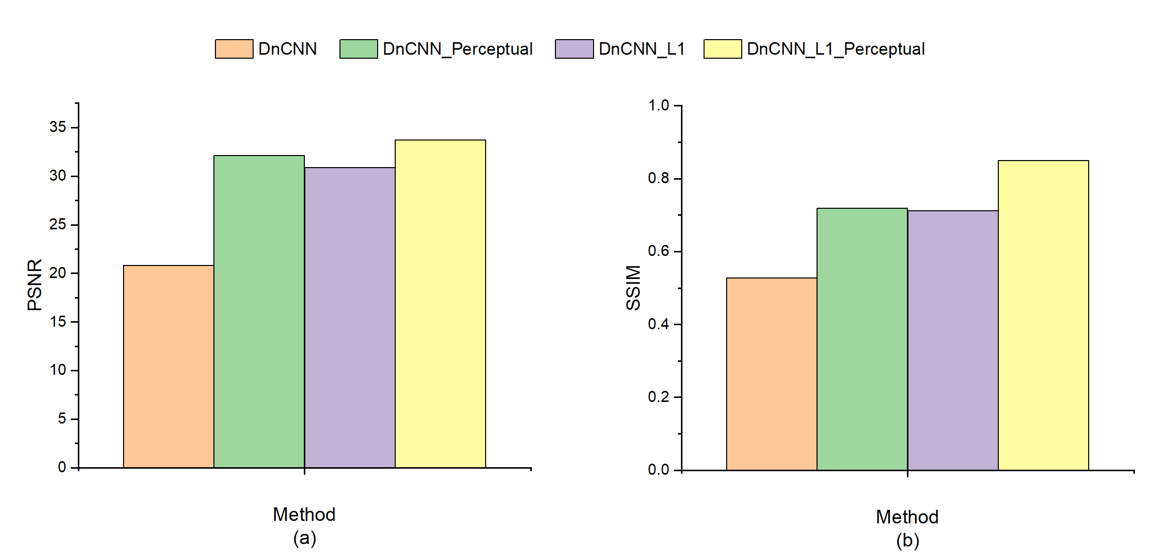
Figure 4: PSNR and SSIM on the test dataset of DnCNN,
DnCNN_Perceptual, DnCNN_L1 and DnCNN_L1_Perceptual.
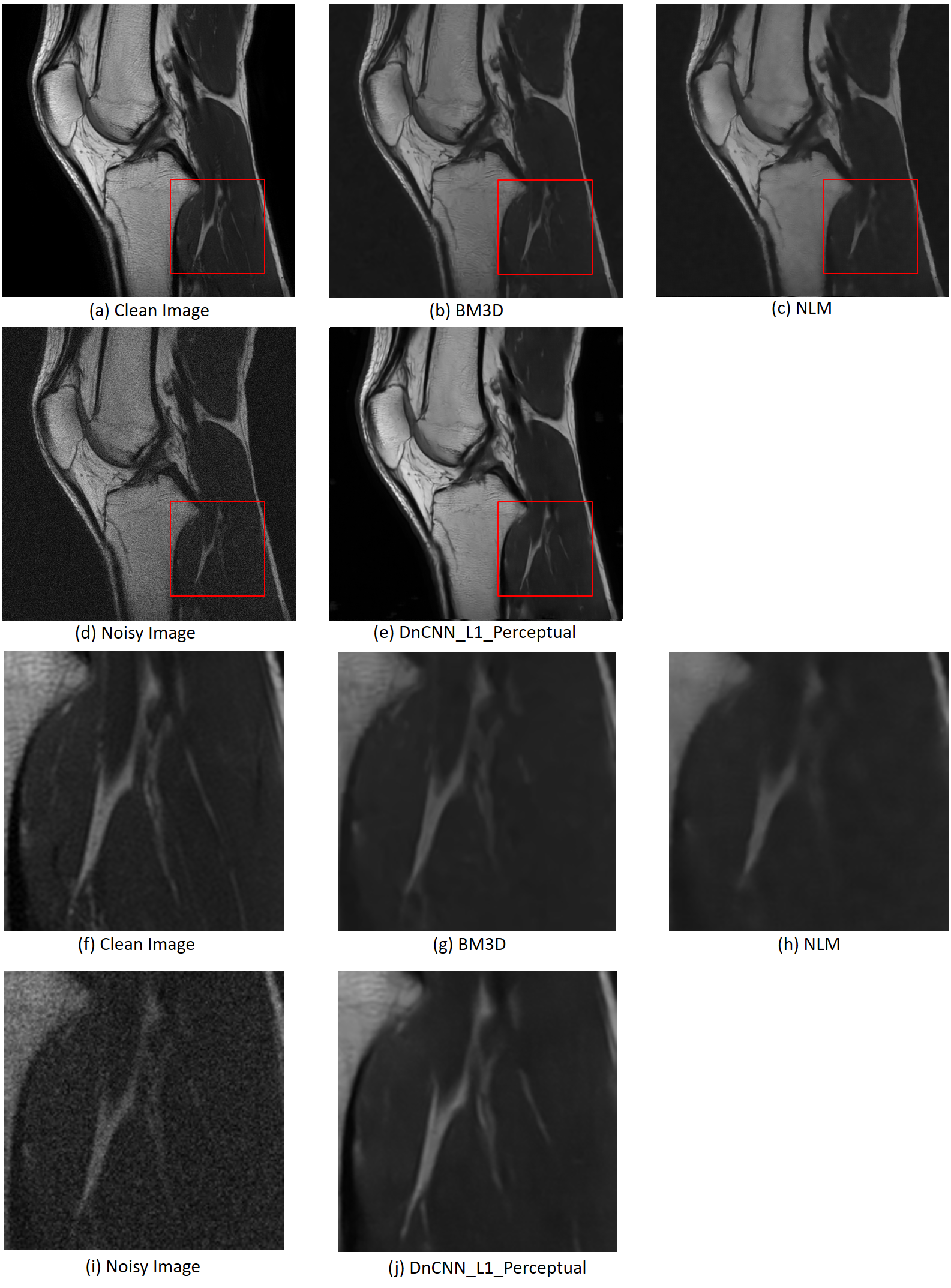
Figure 5: Visual Comparison between clean image, noisy image
and denoised images generated by BM3D, NLM and DnCNN_L1_Perceptual. (a) to (e)
are the images with full FOV. (f) to (j) show the zoom-in region. PSNR and SSIM
of BM3D, NLM, DnCNN_L1_Perceptual concerning these images are (21.11db, 0.58), (20.91db,
0.55) and (33.82db, 0.86) respectively.