3671
Differentiating Predominant Gait Disorder Parkinsonism Using Automated Geometric Indices1Signal Image Processing Group, Singapore BioImaging Consortium, A*STAR, Singapore, Singapore, 2Diagnostic Radiology, Singapore General Hospital, Singapore, Singapore, 3National Neuroscience Institute – SGH Campus, Singapore, Singapore, 4Duke-NUS Medical School, Singapore, Singapore, Singapore
Synopsis
Gait apraxia has attributed to ventriculomegaly and periventricular leukoariaosis. Geometric quantification of ventriculomegaly using Evans’ Index (EI) and Callosal Angle (CA) have been proposed as biomarkers of normal pressure hydrocephalus (NPH). The novel Splenial Angle (SA) may aid in differentiating healthy controls (C) and Parkinson's Disease (P) patients from those with postural instability and gait difficulty (G) subtype and NPH. CA and SA are significantly lower in G patients compared to C and P while EI is significantly higher. Automation of these geometric measures is relatively accurate for EI and SA but further improvements are needed for CA.
Introduction
Gait apraxia in Normal Pressure Hydrocephalus (NPH) is attributed to abnormal build-up of cerebrospinal fluid in the brain's ventricles and periventricular white matter hyperintensities. Parkinsonism gait disorders with ex vacuo ventriculomegly from brain atrophy and leukoariaosis may have overlapping clinico-radiological presentations. Evans' Index (EI),1,2 callosal (CA)3 and splenial (SA)4 angles are useful geometric surrogate measures of ventriculomegaly in NPH, but may be variable without training to improve accuracy and reliability.4-6 EI is a gross, nonspecific marker of ventriculomegaly.1,2 CA is useful in patient selection for shunt surgery in NPH3 and differentiating NPH from other neurodegenerative disorders such as Alzheimer’s disease.7 SA is a novel angular index of ventriculomegaly on axial fractional anisotropic map of diffusion tensor Imaging.4 The aims of this work are to (1) design and implement automated geometric measurements of EI, CA and SA, (2) compare them with ground truth manual measurements, and (3) assess the utility of the automated measures in classifying and identifying predominant gait disorder subgroup of Parkinsonism.Method
Approval from the institutional ethics committee for this study and informed consent from 64 subjects: healthy controls (C) (n = 19), patients with idiopathic Parkinson’s disease (P) (n = 21) and the postural instability and gait difficulty motor subtype (G) (n=24) were obtained. Patients were diagnosed by a movement disorders neurologist in a tertiary referral center using established clinical criteria from the United Kingdom PD Brain Bank8 and DATATOP.9 Brain MRI was performed on a 3T scanner, and images from the sagittal 3D magnetization-prepared rapid gradient echo (MPRAGE) structural brain scan (TR/TE/TI/FA 2200/3.0/900ms/9o; FOV 240mm; matrix 256×256; slice thickness 0.9mm, 192 slices) used for automation of the geometric indices. The MR brain images were registered to MNI space, skull stripped with deepbrain10, and segmented using Multi-Atlas Label Propagation with EM-refinement (MALPEM)11, followed by mask extraction of left and right lateral ventricles for geometric measurements. All automation was done in MATLAB. EI is defined as the ratio of maximum width of the frontal horns of the lateral ventricles and maximal internal diameter of brain. The measurements were taken from the axial slice of lateral ventricles mask and the brain mask (Figure 1A). For CA calculation, bounding box(es) were placed on coronal slices (perpendicular to the anterior-posterior commissural, AC-PC, plane) through the lateral ventricle masks and angle calculated between two tangents formed in between corpus callosum (cc) and ventricles by using inverse cosine (Figure 1B). The overall CA is an average of the angles measured on PC ± one slice. For SA calculation, bounding box(es) were placed on axial slices parallel to the AC-PC plane though the lateral ventricle masks and angle calculated between two tangents formed in between splenium of cc and ventricles by using inverse cosine (Figure 1C). The slice for calculation of SA is identified by calculating the lateral ventricle height and its midpoint on the coronal plane at PC. The overall SA is an average of the angles measured on slice of interest ± one. MedCalc statistical software was used to construct Bland-Altman plots to compare the accuracy of the automated measurements with respect to ground truth. Unpaired Two-Samples Wilcoxon Test was conducted to compare the measurements (EI, CA and SA) between groups (C, P and G). K-means clustering was performed using EI, CA and SA as features to explore the natural clusters among different subject cohorts.Results and Discussion
Mean difference between the ground truth and automated measurements for EI and SA were smaller (Figures 2A & C) than CA (Figure 2B). G patient cohort showed significantly smaller CA and SA and significantly larger EI (Figure 3). K-means clustering were performed using one feature, two features and all the three features (Figure 4). Based on cluster 1, for one feature-based classification, CA showed a better separation of G cohort (Figure 4B) whereas in combination of two features i.e. CA combined with either EI or SA, it showed similar separation in terms of number of subjects present in each group (Figures 4D, F). When all the features were combined, similar separation was shown (Figure 4G). Further examination of subject identity showed that those present in cluster 1 on Figure 4B is identical to those on Figures 4D and F. This shows that EI is redundant and CA is useful in the isolation of G patient cohort. Subjects present in cluster 1 on Figure 4F is identical to those present in cluster 1 on Figure 4G. This further shows that EI is redundant in the isolation of G patient cohort. One of the subjects within the G cohort and the only one subject in the P cohort in the cluster on Figure 4G are different from those present in Figure 4G. We could infer that with the addition of SA, it helped to make the separation of the clusters more robust. In conclusion, CA and SA measurements are helpful in differentiating G patients from C and P patients. For future work, we could implement these automated geometric measures for NPH detection, quantify disease severity for shunt surgery selection and compare these measures pre and post-shunt after further algorithm fine-tuning in order to increase measurement accuracy.Acknowledgements
This study was funded through a research grant from the National Medical Research Council (Singapore).References
1. Relkin N, Marmarou A, Klinge P, et al. Diagnosing idiopathic normal-pressure hydrocephalus. Neurosurgery. 2005;57(3 Suppl):S4-16; discussion ii-v. PubMed PMID: 16160425.
2. Mori E, Ishikawa M, Kato T, et al. Guidelines for management of idiopathic normal pressure hydrocephalus: second edition. Neurol Med Chir (Tokyo). 2012;52(11):775-809. Epub 2012/11/28. PubMed PMID: 23183074.
3. Virhammar, Johan, et al. The callosal angle measured on MRI as a predictor of outcome in idiopathic normal-pressure hydrocephalus. J Neurosurg. 2014;120:178–184
4. LL Chan, Chen RC, WY Go, et al. The Splenial Angle: A Novel Index in Idiopathic Normal Pressure Hydrocephalus. 27th Annual Meeting of the International Society of the Magnetic Resonance in Medicine, Montréal, QC, Canada, 11-16 May 2019.
5. Weerakkody Y, Venkatesh M, et al. Evans' index. https://radiopaedia.org/articles/evans-index-1. Accessed October 27, 2019.
6. W Lee, A Lee, R Chen, N Keong, LL Chan. Improving the accuracy of callosal angle measurement in diagnosis of normal pressure hydrocephalus. 36th Annual Scientific Meeting of the European Society for Magnetic Resonance in Medicine and Biology, Rotterdam, Netherlands, 3-5 Oct 2019.
7. Cagnin, Annachiara, et al. A simplified callosal angle measure best differentiates idiopathic-normal pressure hydrocephalus from neurodegenerative dementia. Journal of Alzheimer's Disease 46.4 (2015): 1033-1038.
8. https://www.parkinsons.org.uk/research/parkinsons-uk-brain-bank
9. DATATOP: A Multicenter Controlled Clinical Trial in Early Parkinson's Disease: Parkinson Study Group. Arch Neurol. 1989;46(10):1052–1060. doi:10.1001/archneur.1989.00520460028009
10. https://pypi.org/project/deepbrain/
11. C. Ledig, R. A. Heckemann, A. Hammers, J. C. Lopez, V. F. J. Newcombe, A. Makropoulos, J. Loejoenen, D. Menon and D. Rueckert, “Robust whole-brain segmentation: application to traumatic brain injury,” Medical Image Analysis, 21(1), pp. 40-58, 2015
Figures
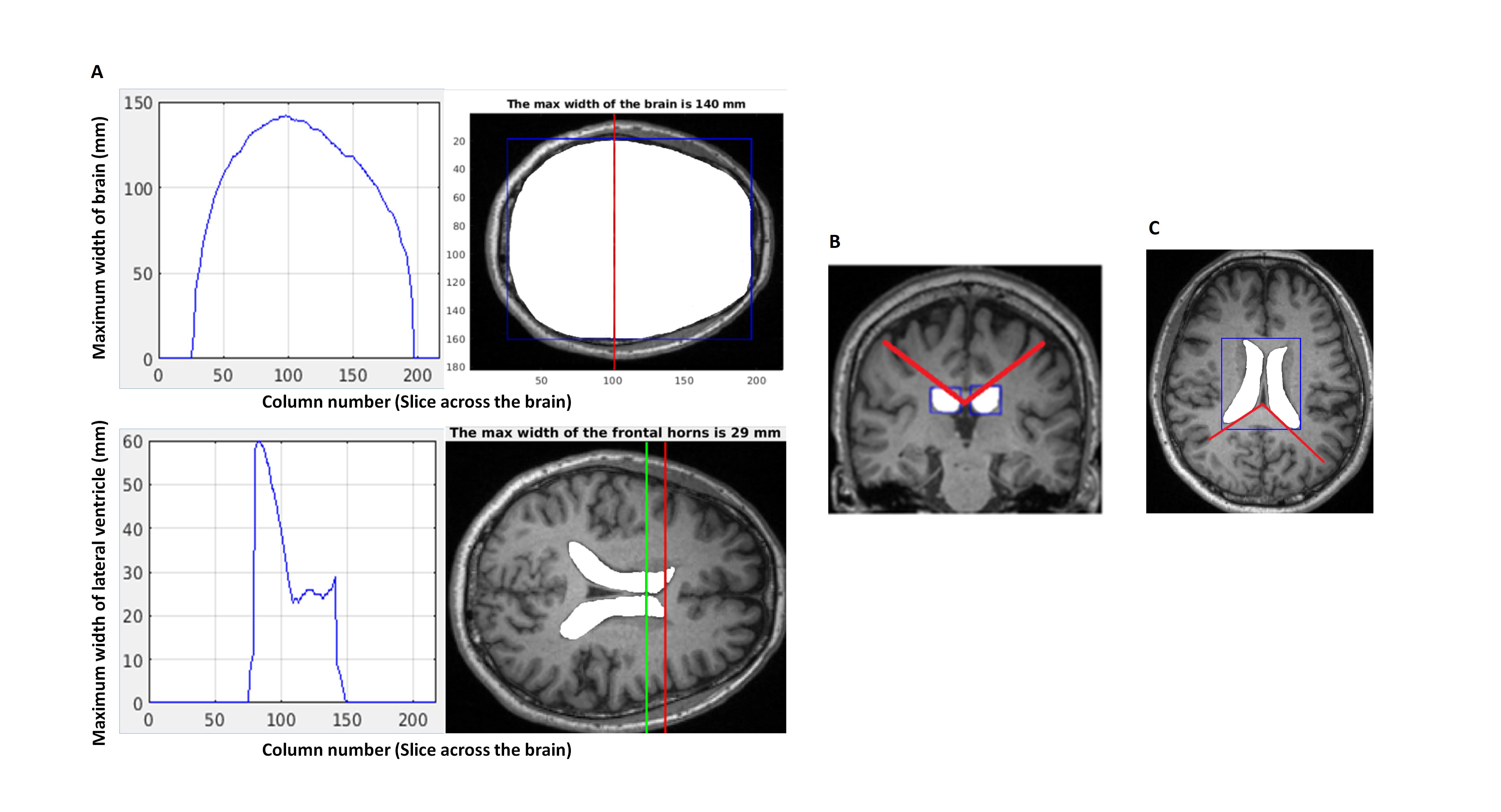
Figure 1 | Annotations where EI, CA and SA measurements were taken
A. Top left plot shows the maximum width of brain against all slices of axial section of brain mask overlaid on MR image shown on the right. Red line within the bounding box depicts the maximum width calculated. Bottom left plot shows the maximum width of the lateral ventricles on the same axial slice as the brain mask. The corresponding ventricle mask overlaid on MR image is shown on the right; Red line depicts the maximum width of frontal horns within the mask
B. CA measured between the red lines
C. SA measured between the red lines
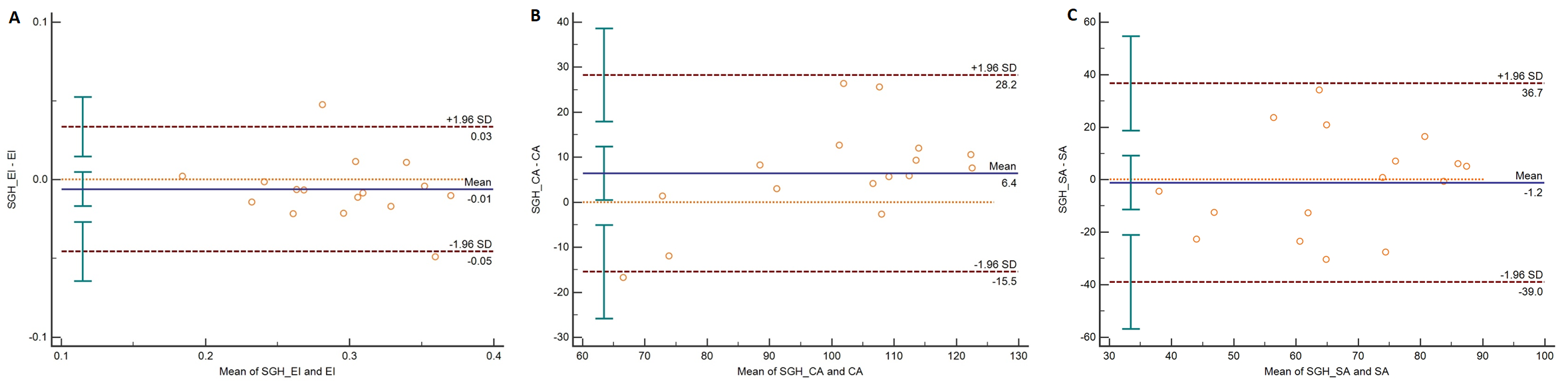
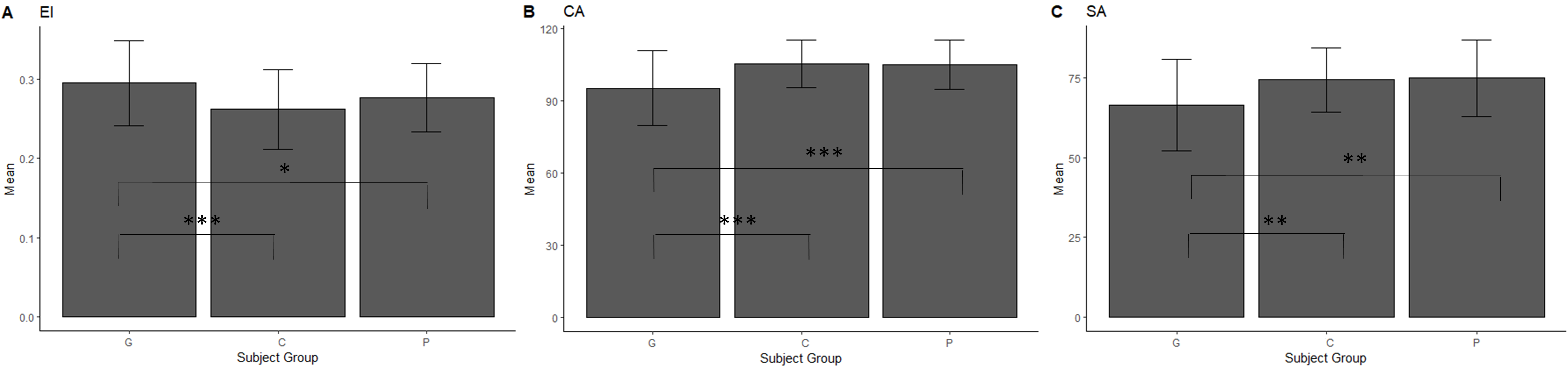
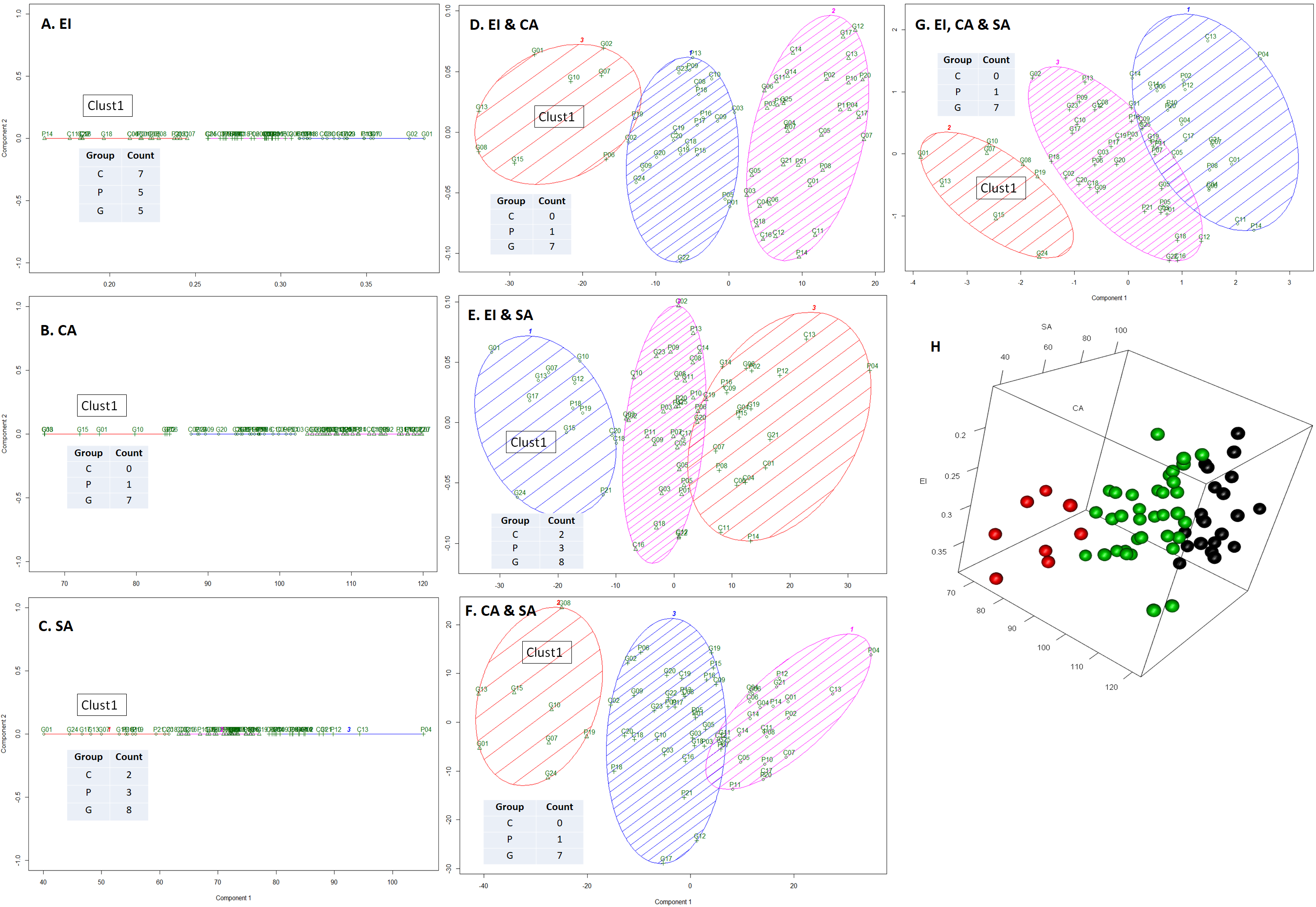
Figure 4 | Classification of subjects based on geometric measures (ID, 2D, 3D) by using K-means clustering. The count of each subject belonging to one of the three groups in the smallest cluster (Clust1) is shown on the table inside each plot.
A-C: Classification of subjects by using EI (A), CA (B) and SA (C)
D-F: Classification of subjects by combining EI with CA (A), EI with SA (B) and CA with SA (C)
G: Classification of subjects by using the three measurements
H: 3D representation of plot shown in G