3665
Complex semi-quantitative noise analysis for single set of MR images1UIH America, Inc., Houston, TX, United States, 2United Imaging Healthcare, Shanghai, China
Synopsis
We propose a noise analysis method based on complex MRI signals. By actively inducing concomitant fluctuation into a single complex MR image, an abrupt change in a predefined signal function (e.g. signal ratio) is observed when signal intensity becomes stronger than background noise. The method is very sensitive to the existence of weak signal such as tissue-background boundaries or very low signal tissues, and can be used to semi-quantitatively distinghuish regions of signal and noise.
Introduction
In the context of MRI, the definition and analysis of noise are generally based on real values1,2, predominantly the signal magnitude. Converting signal from complex to real may modify noise behavior, especially for pure noise which is Gaussian in complex but Rician in magnitude3. Therefore it would be beneficial to evaluate noise in complex domain.When repeated scans are not feasible such as unacceptable scanning time, the option for noise evaluation is generally limited. Most often a spatial sliding window is used to determine signal variation in neighboring voxels, which is subject to errors especially at tissue boundaries. Or one can make use of the signals from multiple coil channels4, which requires sophisticated algorithm and noise model.
In this works, we will demonstrate that, by introducing a concomitant fluctuation into a single complex MR image, as well as using a multi-dimensional integration5 (MDI) strategy, a semi-quantitative noise probability index can be calculated to distinguish between signals and noise.
Methods
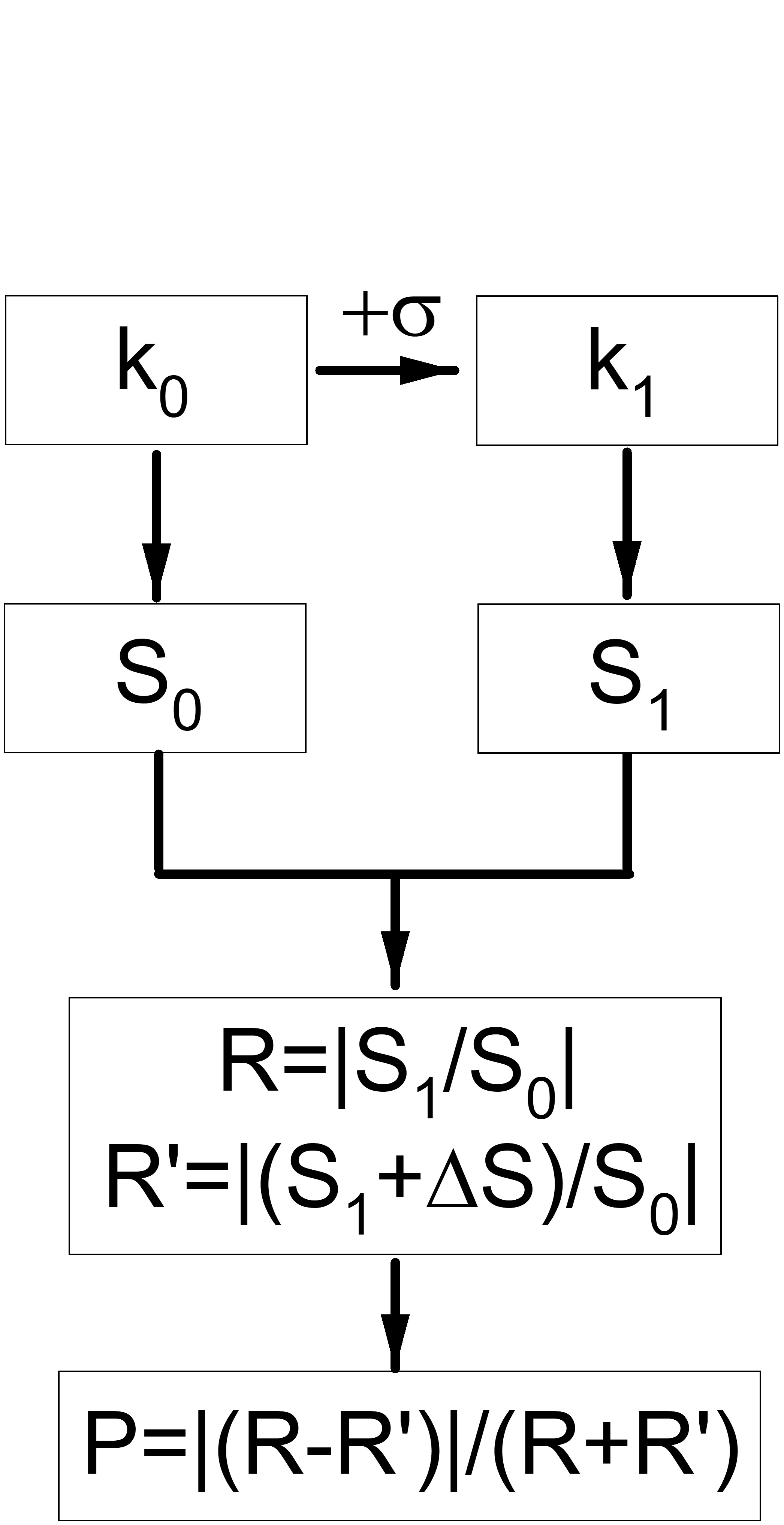
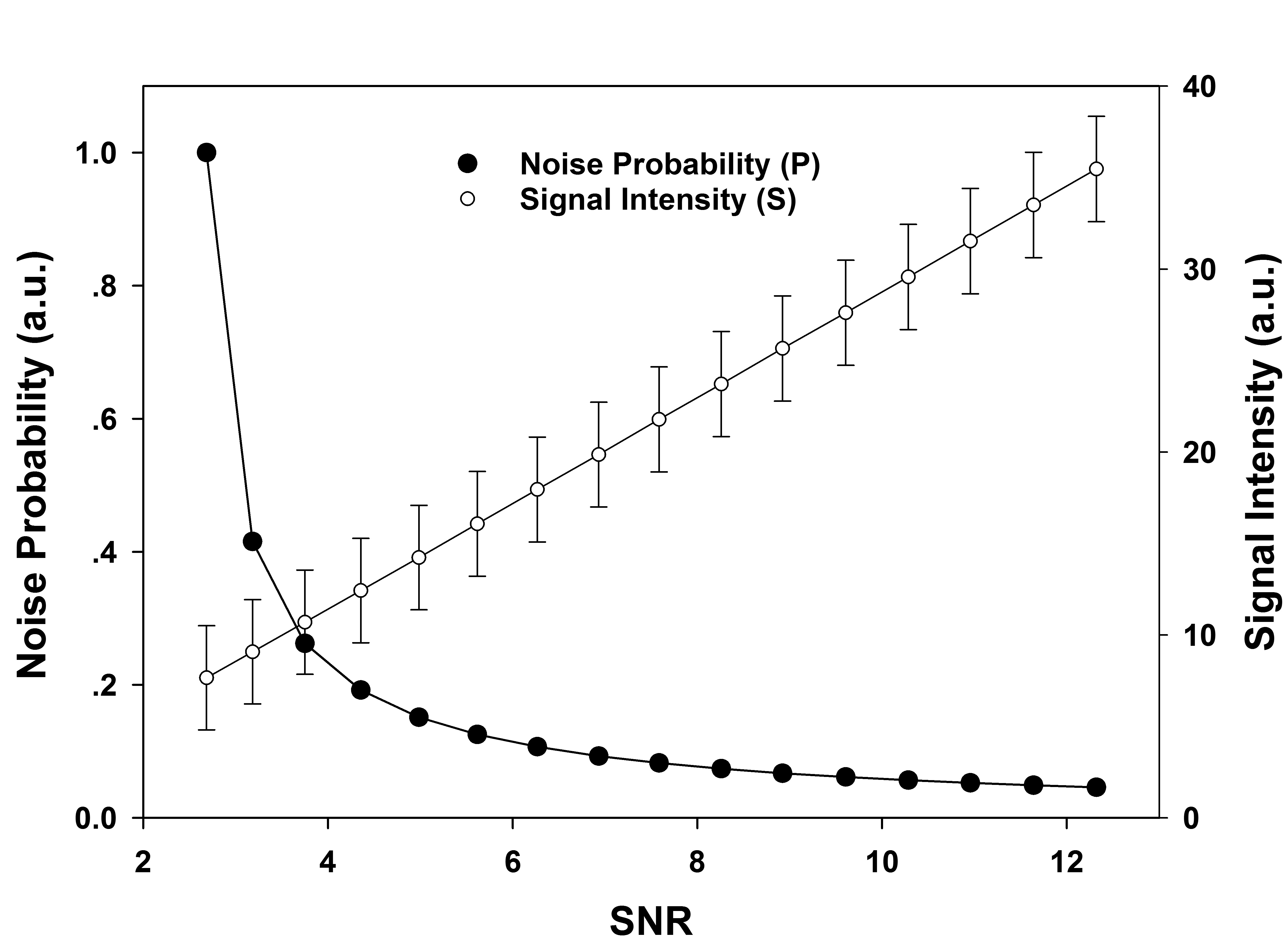
The proposed noise evaluation procedure is shown in Fig.1. The original k-space k0 is added with complex noise to create k1, both of which lead to S0 and S1. The added complex noise is Gaussian with a small variation σ. Then two signal ratios can be defined as $$$R=S_{1}/S_{0}$$$ and $$$R'=(S_{1}+\Delta S)/S_{0}$$$. ΔS can be set as such that it is small relative to signal, but large relative to noise. Finally a noise probability index is defined as $$$P=|R-R’|/|R+R’|$$$. P is expected to be about 1 for pure noise, and about 0 for very high signals. For best outcomes with MDI, coil uncombined complex data were used5.For Monte Carlo simulation, σ was set to 1 for both real and imaginary parts, while signal intensity varied from 0 to 12, leading to a SNR range of about 2~12. The mean signal intensity 6 was used as ΔS. The process was repeated 105 times to determine the averaged SNR, signal mean and variation, as well as the corresponding P.
For MR imaging, 3D GRE brain data were obtained at 3T (uMR790, UIH, China) with TE/TR=4.3/10ms, FA=16°, voxel size=1x1x2mm3 and 24 channel head coil. Firstly, full k-spaces (k0) of individual channels were reconstructed and added with noise (k1), each correspond to S0 and S1, respectively. The added noise to k1 was based on the overall noise level estimated from S0. Thirdly, on a voxel-by-voxel basis, S0 was normalized by the mean signal of the whole image, and ΔS was estimated by dividing the overall noise by the normalized S0. MDI was adopted to calculate R and R’ by solving the following problems:
$$ min_{R}\sum_1^{N_{c}}||\frac{S_{1}}{S_{0}}-R||_2^2 $$
$$ min_{R'}\sum_1^{N_{c}}||\frac{(S_{1}+\Delta S)}{S_{0}}-R'||_2^2 $$
Where Nc is channel number of the head coil.
Finally, the noise probability map is calculated as described above.
Results
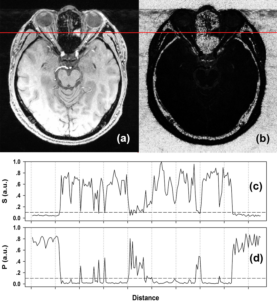
The simulated signal intensity and noise probability as functions of signal SNR are shown in Fig.2. As expected, the signal intensity curve was linearly ascending as a function of SNR. However, the noise probability was nonlinearly related to SNR, with a sharp descent from 1.0 to around 0.2 at low SNR regime dominated by noise, while coming to a flat curve with very slow decay under 0.2 in high SNR regime, where signal had become significantly stronger than noise. Fig.3 displays a typical coil combined (using SOS) GRE image (Fig.3a) and its corresponding noise probability map (Fig.3b). Visually, the noise probability map resembles an inverse of the original image contrast. Quantitatively, however, the signal (Fig.3c) and noise probability (Fig.3d) profile (red lines in Figs.3a & 3b) revealed that the latter nonlinearly amplified noise regions and suppressed tissue regions, indicating a sensitive semi-quantitative representation of SNR.Discussion
Numerous efforts have been dedicated to noise analysis of MR images6-9. In this work, we propose a simple yet sensitive estimation of the probability of a voxel being noise. By introducing additional noise and signal variation, concomitant differentiated changes can be induced. For voxels with pure noise or weak signal, R is dominated by σ while R’ by ΔS, thus leading to high P values as ΔS >> σ. For voxels with strong signal, both R and R’ are determined by S0, making P close to 0 as ΔS <<S0. Therefore the P index is a nonlinear semi-quantitative measure of SNR.The sensitivity of the proposed noise probability index to very weak signal is due to the fact that it is calculated based on complex signal rather than real signal. Pure Gaussian complex noise has a mean value of 0, and if overlapping with a definitive signal, even as small as σ, the upper limit of R will reduce significantly, and hence the P value is reduced. Moreover, the use of MDI further ensures the reliability of the calculation of P, as utilizing signals from all coils will significantly reduce the chance of a zero divisor in R and R’.
Conclusion
In conclusion, we have demonstrated a semi-quantitative noise analysis method for any single set of complex MRI images. With the use of MDI, the resultant noise sensitivity index is sensitive to very weak signals, and can be used to reliably distinguish between background and objects.Acknowledgements
No acknowledgement found.References
1. Pandian DS, Ciulla C, Haacke EM, Jiang J, Ayaz M. Complex threshold method for identifying pixels that contain predominantly noise in magnetic resonance images. J Magn Reson Imaging 2008;28(3):727-735.
2. Ocali O, Atalar E. Ultimate intrinsic signal-to-noise ratio in MRI. Magn Reson Med 1998;39(3):462-473.
3. Haacke EM, Brown R, Thompson M, Venkatesan R. Magnetic resonance imaging. Physical principles and sequence design. New York: Wiley-Liss; 1999. 32-45 p.
4. Veraart J, Fieremans E, Novikov DS. Diffusion MRI noise mapping using random matrix theory. Magn Reson Med 2016;76(5):1582-1593.
5. Yongquan Y, Jingyuan L. MR Relaxivity Mapping using multi-dimensional integrated (MDI) complex signal ratio. 2019; Montreal. p 1356.
6. Thunberg P, Zetterberg P. Noise distribution in SENSE- and GRAPPA-reconstructed images: a computer simulation study. Magn Reson Imaging 2007;25(7):1089-1094.
7. Ding Y, Ying L, Zhang N, Liang D. Noise behavior of MR brain reconstructions using compressed sensing. Conf Proc IEEE Eng Med Biol Soc 2013;2013:5155-5158.
8. Khan AF, Younis MS, Bajwa KB. Nonlinear Bayesian estimation of BOLD signal under non-Gaussian noise. Comput Math Methods Med 2015;2015:389875.
9. Kidoh M, Shinoda K, Kitajima M, Isogawa K, Nambu M, Uetani H, Morita K, Nakaura T, Tateishi M, Yamashita Y, Yamashita Y. Deep Learning Based Noise Reduction for Brain MR Imaging: Tests on Phantoms and Healthy Volunteers. Magn Reson Med Sci 2019.
Figures