Introduction

Image intensity nonuniformity is a common MRI artifact manifested by variation of signal intensity across the image even within the same tissue. Nonuniformity may be caused by RF field inhomogeneity, inhomogeneous reception coil sensitivity, and patient’s influence on the magnetic and electric field. This artifact is detrimental to tissue segmentation, inter-modality coregistration, parametric mapping, and radiomics analysis, and therefore retrospective correction is often required. Retrospective approaches entail estimating a "smooth" multiplicative bias field B(r) to correct the image (Figure 1). The most commonly used method is the N3 algorithm¹ and its N4 refinement. ² N3/N4 employ an iterative deconvolution that estimates B(r) so as to maximize the high frequency content of the corrected image. In our experience, however, the method does not perform well in challenging imaging situations such as abdominal, ultra-high field or accelerated MRI, and further improvements are necessary. We have implemented a method we call BiCal where, after preprocessing to exclude sharp edges and background region, the bias field is fitted directly. We compared the performance of BiCal to N4 in three challenging applications: abdominal MRI acquired at 3T using accelerated radial GRASP, 3T breast imaging using a dedicated breast coil, and 7T head imaging.

Methods

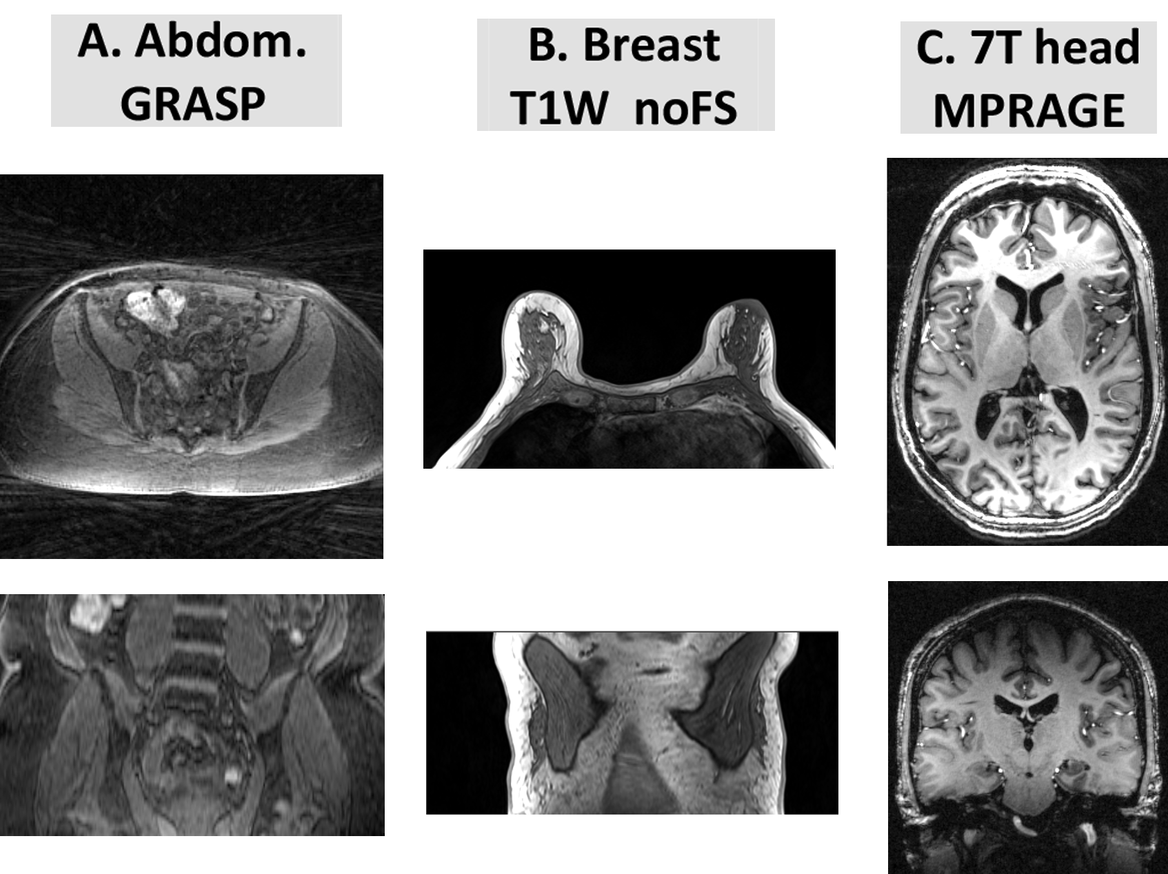
Patient datasets: This was an IRB-approved, retrospective study with waived informed consent. Patient datasets (Figure 2) were randomly selected from image database used in previous clinical research studies ^3,4. (A). Abdominal images were time-frames extracted from dynamic studies acquired using GRASP 3D stack-of-star radial FLASH sequence, TR/TE= .27/1.88 msec, FA=12^o, voxel size =1.5 x 1.5 x 3 mm. Breast images were acquired a 3T Siemens Trio using a seven-element surface breast coil (Sentinelle, Invivo, Gainesville, FL, USA), TR/TE=4.74/1.79 ms, 448 x 358 x 116 matrix. MPRAGE head images (TR/TE/TI=2.6/2600/1100 msec, FA=6°, 346 × 323 x 248 matrix) were acquired on a 7T Siemens magnet and a volume-transmit 24-element receive coil array (Nova Medical, Boston, Mass).
Correction methods: N4 (a variant of N3) expresses the bias field B(r) as a convolution of the intensity histogram by a Gaussian. The computation consists of iterating between deconvolving the intensity histogram by a Gaussian, remapping the intensities, and then spatially smoothing this result by a B-spline model. The executable N4 code ² is called explicitly by our software. BiCal method is implemented in FireVoxel image analysis software from NYU Center for Biomedical Imaging. In BiCal B(r) is estimated as a set of smooth bias functions such as direct cosines or 3D Lagarange polynomials. After preprocessing to remove sharp edges and background (air) signal, the partial derivatives of the bias field are fitted directly to the partial derivatives of the intensity.
Outcome Measure: To quantify nonuniformity before and after correction we used the coefficient of joint variation⁵ (CJV). CJV = (σ₁+σ₂ ) / |μ₁-μ₂|, where μ and σ are the mean and stdev of the intensity of two sets of regions of interest (seeds) placed across the image. CJV quantifies both the intensity variability in each set and controls for the loss of tissue contrast.
Seeds: Four experienced readers independently placed two groups of seeds. In the brain dataset, seeds were placed in white matter and gray matter; in the breast, in fat and fibroglandular tissue (FGT); and in the abdomen, in subcutaneous fat and muscle. Seeds were added incrementally until the change in CJV after the addition of new batch of seeds did not exceed 2.5%. This resulted in the following number of seeds (avg±st dev): in the brain, 194±14 in both white and gray matter; in the breast, 181±71 in fat and 113±49 in FGT; and in the abdomen, 253±102 in fat and 254±104 in muscle.
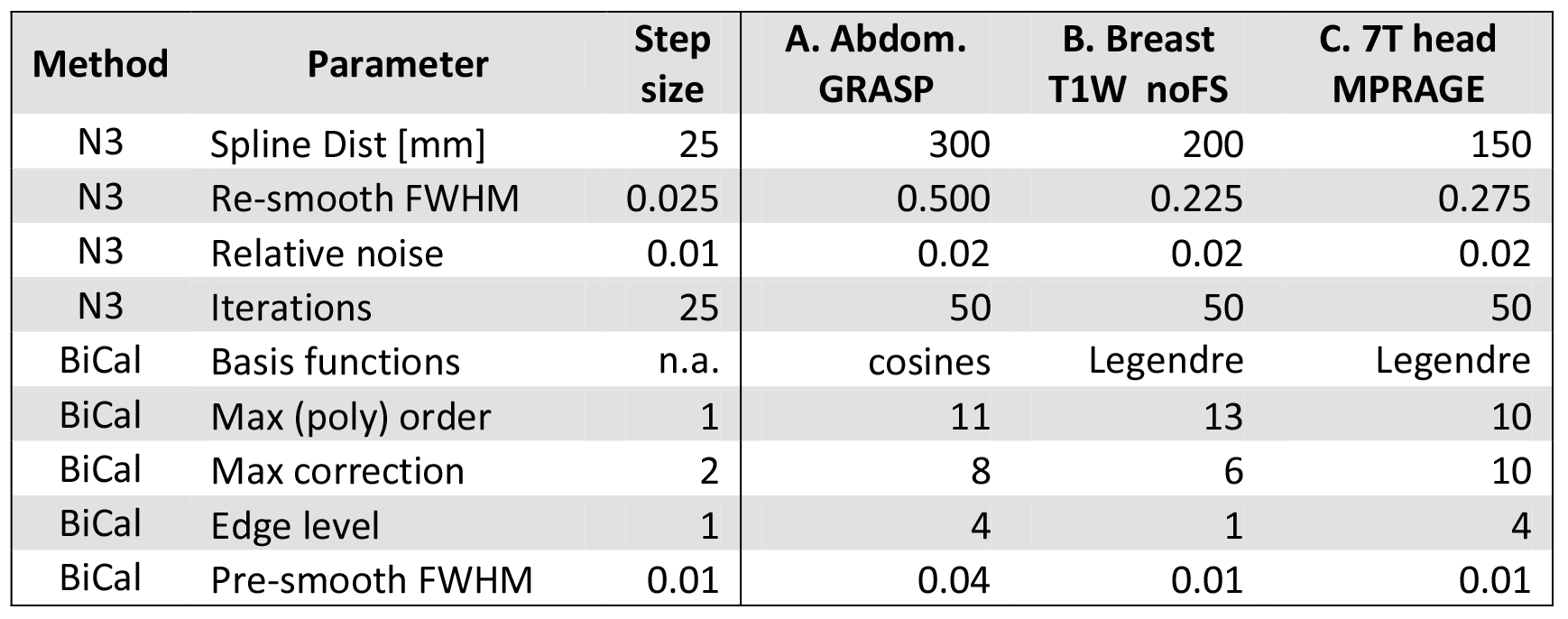
Training and testing: N4 and BiCal were optimized on the randomly selected training datasets. The size of the training set is determined by successive addition of cases and optimizing parameters until the change in average CJV becomes negligible. The optimal parameters (Figure 3) are then used to process an independent set of test cases and compare algorithm performance.

Results

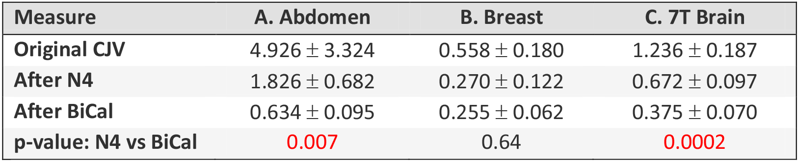
The process of parameter optimization (FIgure 3) successfully converged in 3-4 iterations. The original CJV and its change after correction (Figures 4 and 5) varied significantly across the three applications. The abdominal (A) dataset showed the highest non-uniformity, the breast (B) images were the most uniform, and 7T brain MRIs (C) were in intermediate position. There was a significant improvement for each method and modality as compared with originally acquired image: p<0.001 for (B) and (C), p<0.05 for (A). For modalities A and C, but not for the breast there was a significant advantage of BiCal over N4.

Discussion

Based on CJV, the new BiCal method significantly outperformed the N4 method in the challenging scenario of 7T brain MRI and abdominal GRASP datasets. These two applications had higher original CJV than breast images. This suggests that BiCal is the method of choice for high-field and fast MRI acquisitions.

Acknowledgements

This work was supported by NIH/NIBIB grant U24 EB028980.