3658
Automatic Longitudinal Assessment of Hippocampal Subfields using Multi-Contrast MRI1The University of Queensland, Brisbane, Australia
Synopsis
Characterising longitudinal changes in the subfields of the hippocampus using high-resolution MRI is important for understanding neurological disorders and diseases including Alzheimer’s. Hippocampus subfields are differentially involved in these disorders and can be used as biomarkers for disease. Here, we introduce an automatic longitudinal pipeline for measuring the subfields of the hippocampus (LASHiS). Unlike other longitudinal pipelines, LASHiS harnesses multiple MR contrasts and is therefore more sensitive to changes in these subfields. We compared LASHiS with four other established methods including Freesurfer and found that our method yields higher test-retest reliability and robust Bayesian longitudinal linear mixed effects modelling results.
Introduction
The hippocampus formation is a heterogeneous brain structure that is implicated in memory, psychiatric and neurological disorders including Alzheimer’s Disease1. The volumetric and morphometric examination of hippocampus subfields in a longitudinal manner using in vivo MRI could lead to more sensitive biomarkers for neuropsychiatric disorders1, as the anatomical subregions have different roles in disease progression and detection1. Longitudinal processing allows for increased sensitivity2 due to reduced confounds of inter-subject variability and higher effect-sensitivity than cross-sectional designs. Advances in MRI acquisition techniques and image analysis methods have made automatic segmentation of these subfields possible3, 4.We examined the performance of a new longitudinal pipeline: “Longitudinal Automatic Segmentation of Hippocampus Subfields (LASHiS)” against three published approaches including cross-sectional and longitudinal Freesurfer (Fs) hippocampal subfields (V6.0)4, and ASHS cross-sectional (ASHS Xs)3. Our pipeline segments the hippocampus subfields utilising joint-label fusion 5 to a non-linearly registered6 Single Subject Template in order to treat every time point the same way7. This pipeline (which shares processing and analysis similarities with the ANTs longitudinal cortical thickness pipeline8) produces robust and reliable automatic multi-contrast segmentations of HFS that measure tissue characteristics available in in vivo ultra-high field MRI scans.Method
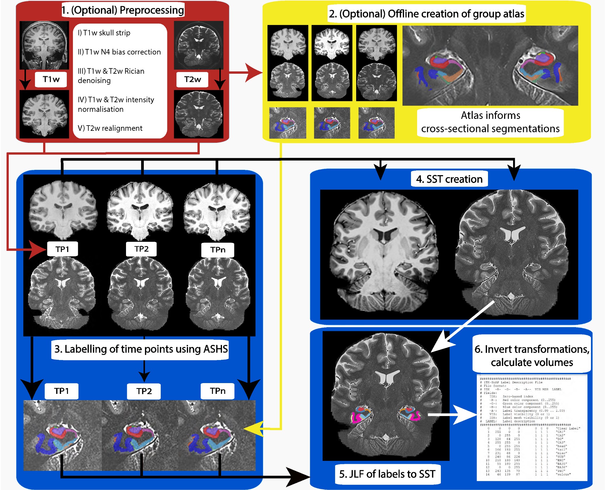
Seven healthy participants (age: M = 26.29, SD = 3.35) were scanned in a 7T whole-body research scanner (Siemens Healthcare, Erlangen, Germany) in three sessions with three years between session one and two, and 45 minutes between two and three. Participants were scanned using a 2D TSE sequence (0.4x0.4x0.8mm3) thrice over a slab planned orthogonally to the hippocampus. A T1w MP2RAGE (0.75mm isotropic voxel size) was also acquired (TR/TE/TIs=4300ms/2.5ms/840,2370ms). TSE images were motion-corrected, resampled to 0.3mm isotropic, Rician denoised, and intensity normalised. The longitudinal pipeline is described fully in Fig. 1.The pipeline consists of the following steps with the input of any number of T1w and T2w individual time points per participant: 1) (In red; optional) preprocessing of both T1w and T2w scans. 2) (In yellow) Offline construction of a sample-specific atlas for LASHiS. 3) Labelling of individual time points of each subject using ASHS and a representative atlas (or an atlas created in 2) to yield hippocampus subfield estimates. 4) Construction of a multi-contrast Single Subject Template (SST). 4) Joint label fusion of each of the individual time point labels to the SST using both contrasts and individual hippocampus subfield labels to produce a labelled SST. 5) Application of the inverse subject-to-SST transformations to SST labels. 6) Measurement and calculation of subfield labels in subject-space.
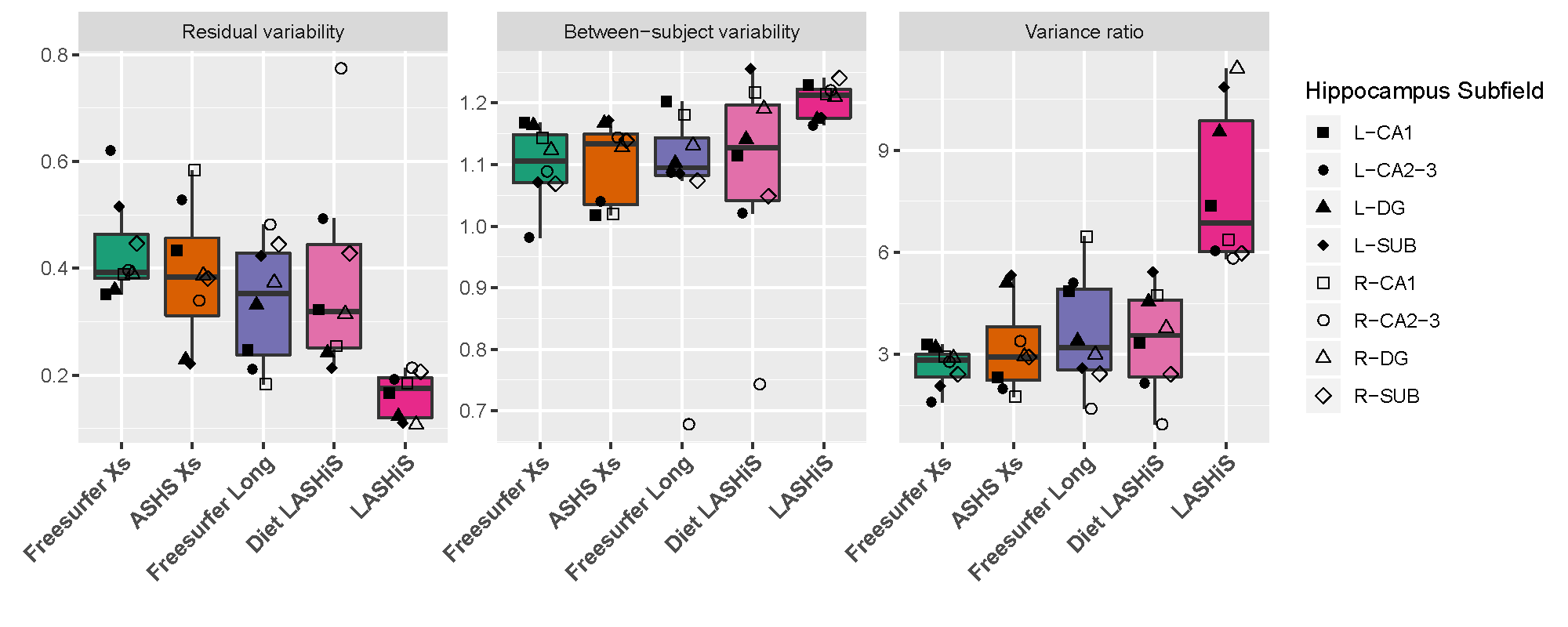
Evaluation of the pipeline was conducted first by test-retest reliability analysis between Freesurfer variants, ASHS Xs, and LASHiS (Fig 2). We then conducted a longitudinal Bayesian Linear Mixed Effects (LME) analysis9 to assess relationships between cross-sectional and longitudinal results while accounting for subject-specific trends8. Specifically, we quantify between, and within (residual) variability of hippocampus subfield volume normalised by total hippocampus subfield volume. It was assumed that the best performing method maximises both within-subject reproducibility and between-subjects variability (to distinguish between sub-groups). Therefore, a variance ratio with greater between-subject variability, and lower residual variability, provides a useful measure of performance for longitudinal pipelines8.
Results
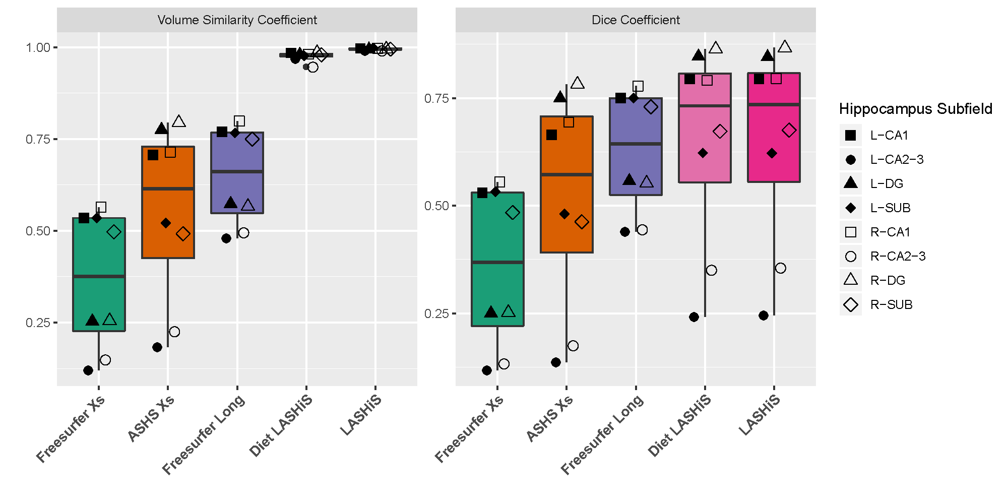
Test-retest results showed that LASHiS produces significantly higher volume similarity and Dice overlaps over time-points compared to Freesurfer and ASHS Xs for all subfields (Fig 3). Freesurfer Xs, ASHS Xs, Diet LASHiS and LASHiS all require resampling to a common space before overlap calculation of Dice overlaps. Higher scores between time-points denote higher subfield overlap between test-retest time-points.We compared the performance of four hippocampus subfield segmentation processing approaches using LME to quantify between and residual variability and the variance ratio between these. We found overlapping confidence intervals for all pipelines. The relative distributions of variability in Fig. 4 show a trend towards higher variance ratios for LASHiS compared to the other methods. Lower residual, and higher between-subject variabilities are preferred for longitudinal pipelines. The variance ratio is a summary statistic of the two variability values, with higher values indicating improved discrimination between within- and between-subject variance.
Discussion and conclusion
Here we present a technique for automatically segmenting hippocampus subfields using high resolution multi-contrast MRI that robustly generates estimates of hippocampus volume in healthy subjects. In the Freesurfer longitudinal scheme, only a T1w scan of an individual is processed through the longitudinal stream of ‘recon-all’ before longitudinal processing of hippocampus subfields, potentially explaining the Freesurfer results. Our design utilises multi-contrast information from a dedicated hippocampus sequence and a standard T1w scan.The design of our pipeline decreases random variability in any session due to the single-subject template registration and joint label fusion labelling scheme. A limitation of our scheme is that joint-label fusion computes weights independently, ignoring that label errors (i.e., systematic errors) in subjects will propagate to the template.
These systematic errors can be avoided through quality assurance of scans and labels. We report only seven participants here, although Bayesian LME is robust to small sample sizes9. To further test the performance of LASHiS we are currently performing analysis on data sets with larger cohorts, e.g., the ADNI3 dataset11.
Acknowledgements
The authors acknowledge the facilities and scientific and technical assistance of the National Imaging Facility, a National Collaborative Research Infrastructure Strategy (NCRIS) capability, at the Centre for Advanced Imaging, The University of Queensland. MB acknowledges funding from Australian Research Council Future Fellowship grant FT140100865. This research was undertaken with the assistance of resources and services from the Queensland Cyber Infrastructure Foundation (QCIF).References
1 A. Maruszak and S. Thuret, “Why looking at the whole hippocampus is not enough—a critical role for anteroposterior axis, subfield and activation analyses to enhance predictive value of hippocampal changes for Alzheimer’s disease diagnosis,” Front Cell Neurosci, vol. 8, Mar. 2014.
2 G. M. Fitzmaurice, N. M. Laird, and J. H. Ware, Applied Longitudinal Analysis. Chicester, UNITED STATES: John Wiley & Sons, Incorporated, 2011.
3 P. A. Yushkevich et al., “Automated volumetry and regional thickness analysis of hippocampal subfields and medial temporal cortical structures in mild cognitive impairment,” Hum Brain Mapp, vol. 36, no. 1, pp. 258–287, Jan. 2015.
4 J. E. Iglesias, K. Van Leemput, J. Augustinack, R. Insausti, B. Fischl, and M. Reuter, “Bayesian longitudinal segmentation of hippocampal substructures in brain MRI using subject-specific atlases,” NeuroImage, vol. 141, pp. 542–555, Nov. 2016.
5 H. Wang, J. W. Suh, S. R. Das, J. B. Pluta, C. Craige, and P. A. Yushkevich, “Multi-Atlas Segmentation with Joint Label Fusion,” IEEE Trans Pattern Anal Mach Intell, vol. 35, no. 3, pp. 611–623, Mar. 2013.
6 B. B. Avants, C. L. Epstein, M. Grossman, and J. C. Gee, “Symmetric Diffeomorphic Image Registration with Cross-Correlation: Evaluating Automated Labeling of Elderly and Neurodegenerative Brain,” Med Image Anal, vol. 12, no. 1, p. 26 41, Feb. 2008.
7 M. Reuter, N. J. Schmansky, H. D. Rosas, and B. Fischl, “Within-subject template estimation for unbiased longitudinal image analysis,” NeuroImage, vol. 61, no. 4, pp. 1402–1418, Jul. 2012.
8 N. J. Tustison et al., “The ANTs Longitudinal Cortical Thickness Pipeline,” bioRxiv, p. 170209, Jul. 2017.
9 T. Sorensen, S. Hohenstein, and S. Vasishth, “Bayesian linear mixed models using Stan: A tutorial for psychologists, linguists, and cognitive scientists,” The Quantitative Methods for Psychology, vol. 12, no. 3, pp. 175–200, Oct. 2016.
10 L. E. M. Wisse, G. J. Biessels, and M. I. Geerlings, “A Critical Appraisal of the Hippocampal Subfield Segmentation Package in FreeSurfer,” Front Aging Neurosci, vol. 6, Sep. 2014.
11 Petersen, R. C. et al. Alzheimer’s Disease Neuroimaging Initiative (ADNI). Neurology 74, 201–209 (2010).
Figures