3653
Development of a method for Bloch image simulation of living tissues
Katsumi Kose1, Ryoichi Kose1, Yasuhiko Terada2, Daiki Tamada3, and Utaroh Motosugi3
1MRIsimulations, Tokyo, Japan, 2University of Tsukuba, Tsukuba, Japan, 3University of Yamanashi, Chuo, Japan
1MRIsimulations, Tokyo, Japan, 2University of Tsukuba, Tsukuba, Japan, 3University of Yamanashi, Chuo, Japan
Synopsis
A method for Bloch image simulation of living tissues was developed and the simulated results were compared with experiments performed for phantoms including T2* distribution and various chemical components. The Bloch image simulation for living tissues is based on a four-dimensional numerical phantom consisting of spatially defined 3D datasets of proton density, T1, and T2 with spatially homogeneous B0 (frequency) offset. The multiple gradient-echo images reconstructed from the MR signal obtained from the Bloch image simulation of the numerical phantom reproduced experimental results for samples that simulated living tissues.
Introduction
The Bloch image simulator that reproduces the MR imaging process on a digital computer is a promising software tool in many fields of MRI studies1-6. Their usefulness has been demonstrated mostly using numerical phantoms with single frequency resonance lines. However, most living tissues contain many resonance lines that result from various chemical components and locally inhomogeneous static magnetic fields. In this study, we developed a method for Bloch image simulation of living tissues including various chemical components and T2* distribution.Materials and Methods
We prepared two phantoms for experiments performed at 1.5 T and 3 T. The phantom for1.5 T consisted of four materials: CuSO4 doped water, peanut oil, fish sausage, and margarine stored in cylindrical containers (diameter = 21mm; length = 82mm). The phantom for 3 T consisted of seven materials: NiCl2 doped water, peanut oil, fish sausage, margarine, chicken breast, chicken liver, and beef thigh stored in cylindrical containers (diameter = 31mm, length = 110mm). The MRI systems used for the experiments were a home-built digital MRI system using a small horizontal bore (280 mm) 1.5 T superconducting magnet (JMTB–1.5/280/SSE, JASTEC, Kobe, Japan) and a 3.0 T whole body MRI system (SIGNA, Premier, GE Healthcare, Waukesha, WI). The phantoms were imaged using 2D multiple gradient-echo sequences (16 echoes, TR/DTE = 800ms/2.2ms and 200ms/1.384ms for 1.5 and 3 T) and standard SE and fast SE pulse sequences for relaxation time measurements. In addition, a 2D SE chemical shift imaging (CSI) sequence7 (slice thickness = 5 mm, FOV = (64 mm)2, TR/TE = 200ms/10ms) was used for the central axial slice of the phantom at 1.5 T. We used a GPU-optimized Bloch image simulator published in 20175. This simulator can be used for any inhomogeneous static magnetic field defined by a B0 map file. The numerical phantoms to simulate the real phantoms used in the experiments were designed as four-dimensional numerical phantoms consisting of spatially defined 3D (128 × 128 × 32 voxels) datasets for proton density, T1, and T2 with frequency offsets (= homogeneous B0 maps) equally spaced at frequency intervals of 3.05 Hz for 1.5 T and 6.1 Hz for 3 T as shown in Fig.1. Bloch image simulations were repeatedly performed for the 3D spatial distributions with 256 homogeneous frequency (B0) offsets. The total MRI signal was calculated by summing up the MRI signals obtained by the Bloch image simulations performed for the single frequency offsets. Parameters describing the numerical phantoms (amplitudes and line width for Lorentzian functions) were fitted to the experimental results acquired with the multiple gradient-echo sequences at 1.5 T and 3 T. The parameter fitting was performed by repeating the simulation using the hill-climbing algorithm.Results
Figure 2 shows central cross-sections acquired with gradient-echo sequences and relaxation times of the phantoms. These relaxation times were used for the Bloch image simulation of numerical phantoms. Figure 3 shows frequency resolved cross-sectional CSI images measured using the 2D CSI sequence. These images clearly show water or -OH resonance peaks in the doped water, fish sausage, and margarine and fat or -CH2- (methylene) peaks in the peanut oil, fish sausage, and margarine. Figure 4(a) shows frequency spectra obtained from image intensities averaged over small circular ROIs in the CSI dataset. Figure 4(b) shows frequency spectra modeled for Bloch image simulation using multiple Lorentzian functions. Figure 5(a)-(b) and (d)-(e) shows image intensities of the cross-sectional images acquired and simulated with the multiple gradient-echo sequences at 1.5 and 3 T. Figure 5(c) and (f) shows scatterplots for experimentally obtained image intensities and those obtained by the Bloch image simulations. Correlation coefficients for the simulation and experiment at 1.5 T were 0.9992, 0.9960, 0.9968, and 0.9895 for the doped water, peanut oil, fish sausage, and margarine, respectively. Correlation coefficients for the simulation and experiment at 3 T were 0.9982, 0.8636, 0.9967, 0.9405, 0.9981, 0.9985, and 0.9996 for the doped water, peanut oil, fish sausage, margarine, chicken breast, chicken liver, and beef thigh, respectively. The correlation coefficients close to 1.0 show that the numerical phantoms accurately reproduced the behavior of the proton spins of the material in the multiple gradient-echo sequences.Discussion
At 1.5 T, simulation of the multiple gradient-echo imaging sequence using the numerical phantom reproduced the experimental result quite well as shown in Fig.5(c). This result demonstrates validity of the numerical phantom at 1.5 T proposed in Fig.1. However, at 3 T, considerable disagreements between simulation and experiment were observed for peanut oil and margarine. This result show that description of the numerical phantom using Lorentzian function was not appropriate for those materials at 3 T because spectral separation caused by the chemical shift became dominant in their spectra at 3 T. However, good agreements between the simulation and experiment at 3 T for fish sausage, chicken breast, chicken liver, and beef thigh suggest that the description of T2* used in the numerical phantom is accurate for many living tissues because pure multiline materials are rarely observed in living systems. In conclusion, we designed numerical phantoms to simulate living tissues using their NMR spectra and succeeded in reproducing intensity of multiple gradient-echo images.Acknowledgements
No acknowledgement found.References
[1] Stöcker T, Vahedipour K, Pflugfelder D, Shah NJ. High-performance computing MRI simulations. Magn Reson Med 2010;64:186–193. [2] Xanthis CG, Venetis IE, Chalkias AV, Aletras AH. MRISIMUL: A GPU-based parallel approach to MRI simulations. IEEE Trans Med Imaging 2014;33:607–616. [3] Cao Z, Oh S, Sica CT, McGarrity JM, Horan T, Luo W, Collins CM. Bloch-based MRI system simulator considering realistic electromagnetic fields for calculation of signal, noise, and specific absorption rate. Magn Reson Med 2014;72:237–247. [4] Liu F, Velikina JV, Block WF, Kijowski R, Samsonov AA. Fast realistic MRI simulations based on generalized multi-pool exchange tissue model. IEEE Trans Med. Imaging 2017;36:527-537. [5] Kose R, Kose K. BlochSolver: A GPU-optimized fast 3D MRI simulator for experimentally compatible pulse sequences. J Magn Reson 2017;281:51-65. [6] Kose R, Setoi A, Kose K. A fast GPU-optimized 3D MRI simulator for arbitrary k-space sampling. Magn Reson Med Sci, 2019;18:208-218. [7] Brown TR, Kincaid BM, Ugurbil K. NMR chemical-shift imaging in 3 dimensions. Proc Natl Acad Sci USA 1982;79:3523-3526,.Figures
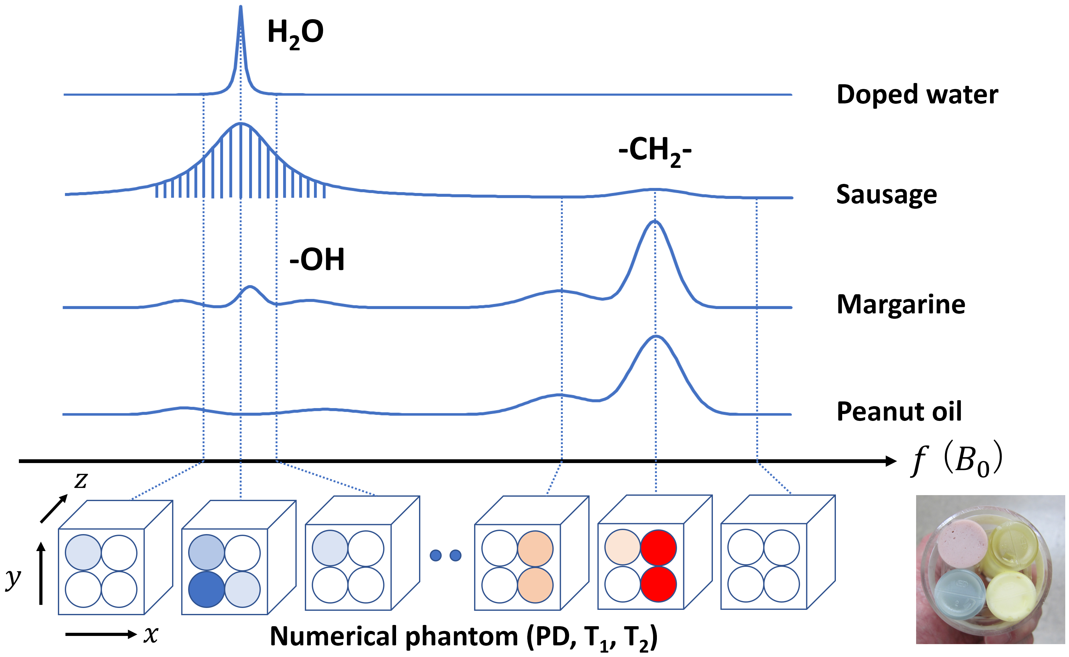
×Numerical
phantom used for Bloch image simulation of T2* and various chemical compositions.
The numerical phantom consists of three-dimensional distributions of proton
density, T1, and T2 with resonance frequencies equally
spaced at frequency intervals of 3.05 Hz for 1.5 T and 6.1 Hz for 3 T. The 3D
phantom consists of 128 × 128 × 32 voxels. The vertical lines in the spectrum of the
sausage schematically show discrete frequency spectrum.
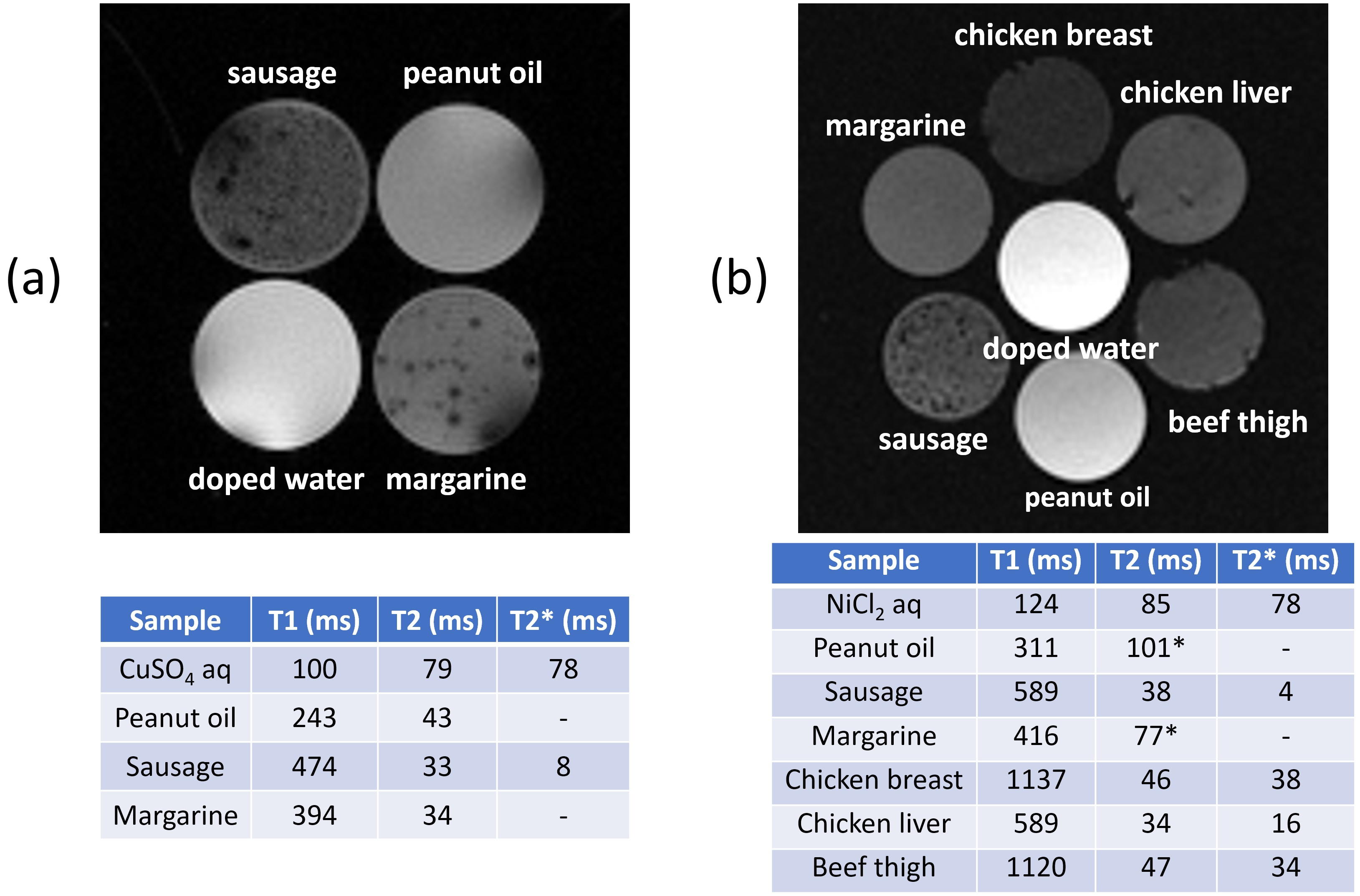
(a)
Upper: the central cross-section of the phantom acquired at 1.5 T using a
gradient-echo sequence (TR/TE = 800ms/4.4ms, FOV = (64 mm)2). Lower:
relaxation times measured using conventional spin-echo and inversion recovery
methods. (b) Upper: the central cross-section of the phantom acquired at 3 T
using a 3D RF spoiled gradient-echo sequence (TR/TE = 13ms/2ms, FOV = (110 mm)2).
Lower: relaxation times measured using conventional methods. Because fast SE
sequences were used, T2 of samples including fat shown by * were
longer than true values.
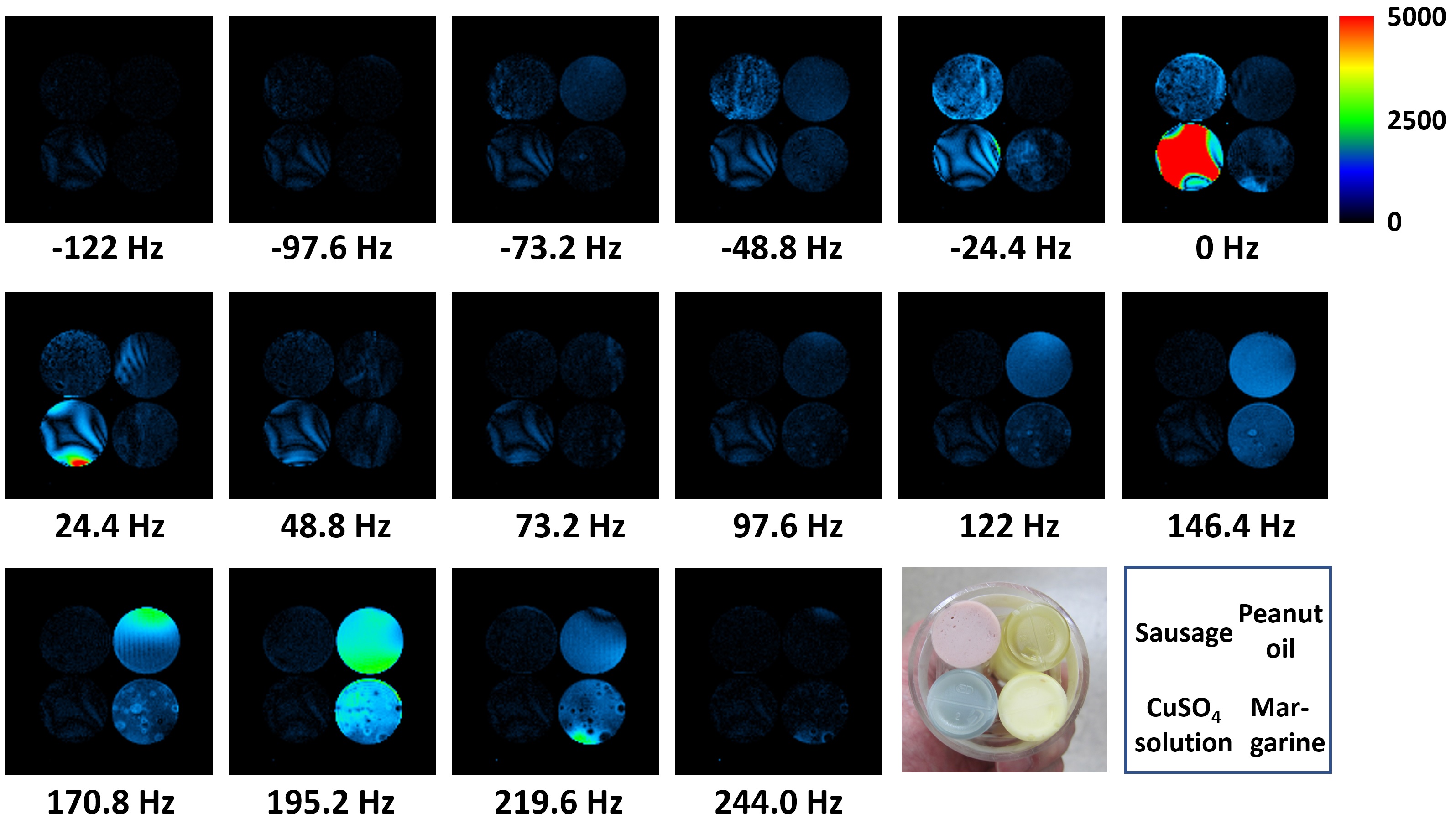
Frequency-resolved
cross-sectional images of the phantom obtained using the chemical shift imaging
sequence at 1.5 T. Slice thickness: 5 mm. FOV: (64 mm)2. In-plane
resolution: 0.5 mm × 0.5
mm. TR: 200 ms. TE: 10 ms. Frequency resolution: 24.4 Hz.
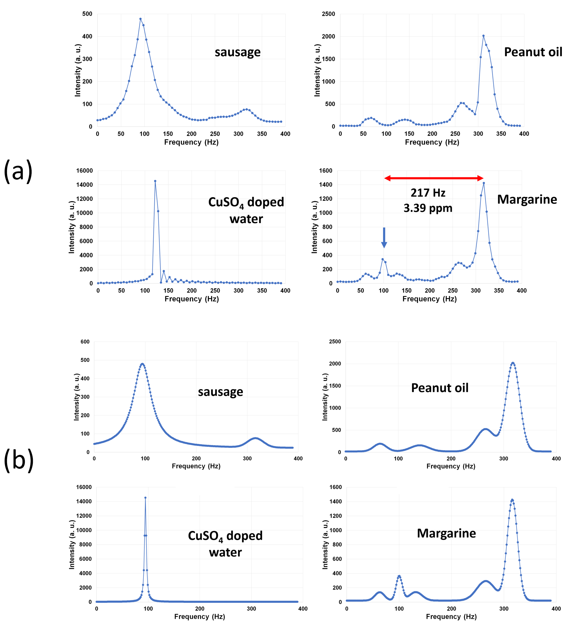
(a)
Frequency spectra obtained from the CSI dataset acquired at 1.5 T. The spectral
intensity was calculated for small circular ROIs in the samples. (b) Frequency
spectra modeled using multiple Lorentzian functions for Bloch image simulation.
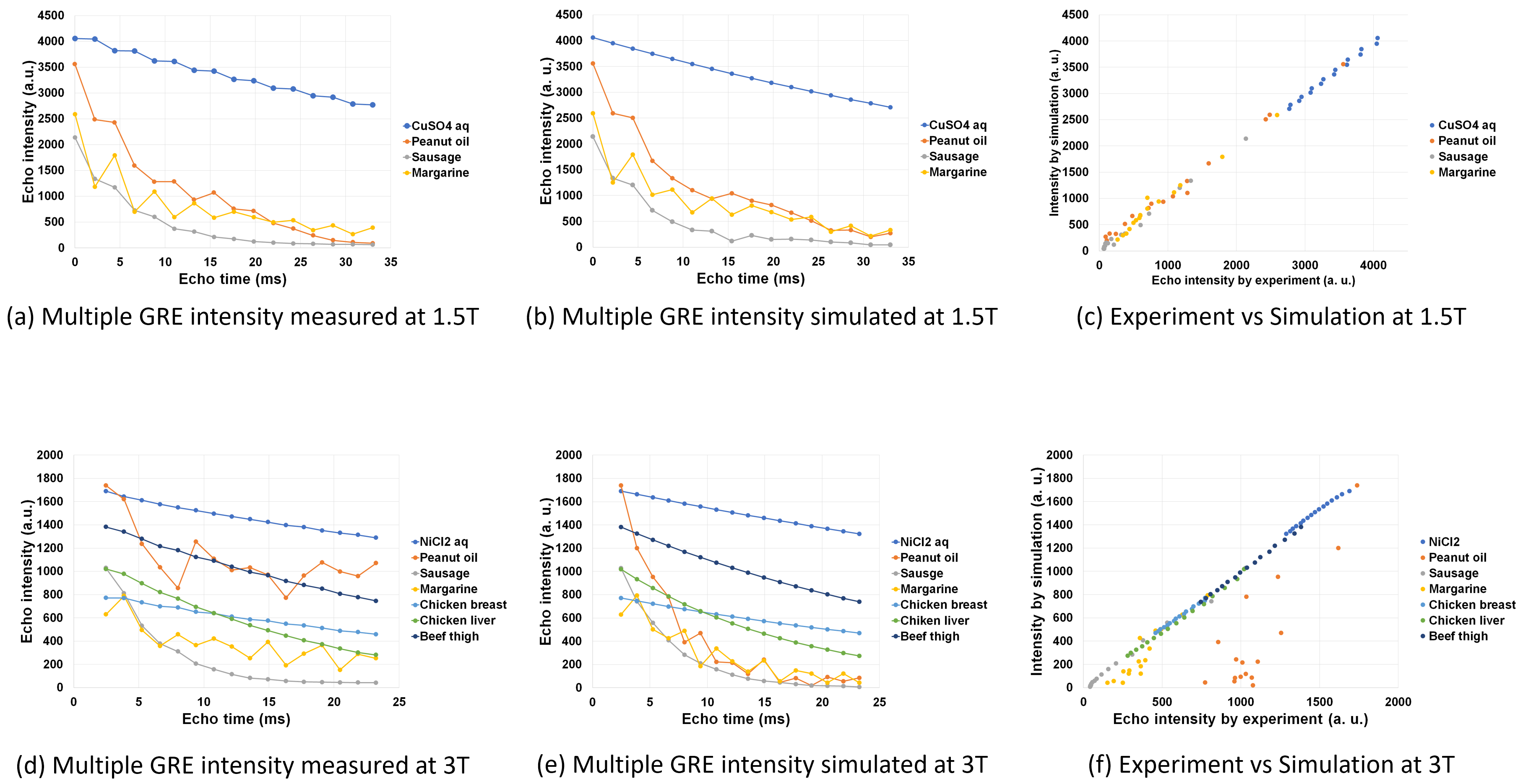
(a)
Intensity of multiple GRE images acquired at 1.5 T. Slice thickness: 5 mm, TR:
800 ms, ΔTE: 2.2
ms. (b) Intensity of multiple GRE images calculated using the numerical
phantom. (c) Scatterplot of the multiple GRE image intensities acquired in the
experiment and the simulation. (d) Intensity of multiple GRE images acquired at
3 T. Slice thickness: 5 mm, TR: 200 ms, ΔTE: 1.384 ms. (e)
Intensity of multiple GRE images calculated using the numerical phantom. (f) Scatterplot
of the multiple GRE image intensities acquired in the experiment and the simulation.