3622
End-to-End Deep Learning Reconstruction for Ultra-Short MRF1Physics, Case Western Reserve University, Cleveland, OH, United States, 2Cardiovascular and Metabolic Sciences, Cleveland Clinic, Cleveland, OH, United States, 3Radiology, University of Michigan, Ann Arbor, Ann Arbor, MI, United States
Synopsis
There are two major challenges in MRF reconstruction, the aliasing artifacts that results from the largely under-sampled k-space, and the very long MRF sequence used in practice to improve the reconstruction accuracy. In this study, we propose an end-to-end deep learning based reconstruction model that aims to address the issue of the spatial aliasing artifacts and provide accurate reconstruction with ultra-short MRF signals.
Introduction
MRF reconstruction is essentially a video-to-image reconstruction. Traditional MRF reconstruction relies on a pre-generated dictionary and pattern matching in the time domain [1]. Recently, some deep learning models have been proposed to replace the dictionary based pattern matching [2]–[4]. However, these models do not directly address the issue of spatial aliasing artifacts caused by largely under-sampled k-space. The pixel-wise temporal signal is distorted by the spatial aliasing artifacts, which will cause mismatches in the recovered tissue parameter maps. In addition, MRF is usually composed of thousands of time frames to improve the reconstruction accuracy. But the relation between the length of MRF sequence and the reconstruction accuracy is inexplicit and largely dependent upon the flip angle sequence. The aim of this study is to deploy a deep neural network structure U-Net [5], [6] and build an end-to-end model that provides artifact-free, fast and accurate MRF reconstruction. Different from similar studies [7], [8], we demonstrate a reconstruction scheme with ultra-short MRF.Methods
We propose a modified U-Net structure to predict tissue parameter maps from the MRF signal evolution. The model structure is detailed in Figure 1. The loss function is the mean square error (MSE) with Adam optimizer and a learning rate of 1e-4. The training program is written in Python with the Keras package and computed on four NVIDIA K80 12G memory GPUs. The neural network model inputs gridded 3D spatial-temporal MRF signal data and directly outputs the tissue parameter T1 or T2 map. The ground truth parameter maps were acquired from a previous study by Eck et al. [9], which consists of 38 in-vivo brain MRF scan images on five subjects and two different MRI machines with the same MRF experiment setup. The aliasing artifacts are synthesized with sparse k-space with an overall under-sampling rate of 10 [Figure2]. Conventionally, in MRF, k-space would be fully covered after a number of TR cycles and all the k-space would be evenly sampled over time. But because an ultra-short MRF sequence is used in this study, random k-space coverage is chosen to avoid uneven coverage of the k-space despite its drawbacks in general MRI applications. The k-space is fully covered at the center and randomly under-sampled on the outside. The random pattern varies between different time frames. A FISP-MRF scheme [10] is adopted with the TR around 8 ms and flip angle (FA) smoothly increasing from 4 degrees to 11 degrees. The synthesized MRF signal consists of only 25 time frames. The dataset with 38 examples is split into 30 for training and 8 for testing. Early stopping is used to prevent overfitting. The reconstructed parameter maps are evaluated by three full-reference metrics: mean squared error (MSE), peak signal-to-noise ratio (pSNR), and structural similarity (SSIM). MSE is used as the loss in the deep learning model and is a direct measurement of accuracy. pSNR and SSIM are metrics to assess the perceived quality.Results
The quality of the deep-learning-based reconstruction is compared to the dictionary-based reconstruction as well as the ground truth parameter maps. The reconstructed maps as well as the residue maps from both reconstruction methods are presented in Figure 3, where the residue map is defined as the absolute difference between a reconstructed map and its corresponding ground truth map. Image quality evaluations for the reconstructed tissue parameter maps versus the corresponding individual examples in the dataset are shown in Figure 4. All three evaluation metrics are similarity metrics in reference to the ground truth maps. The average numbers of the evaluations are listed in Table 1.Discussion and Conclusion
The end-to-end deep learning based reconstruction shows great advantage over dictionary based matching in both T1 and T2 maps. The U-Net predicted T1 and T2 maps present much sharper edges and more detailed structures than the dictionary based reconstruction. In addition, there is also significantly less residue in the U-Net predicted maps. The quantitative assessment is consistent with the visual perception. The U-Net prediction outperforms dictionary based reconstruction in terms of MSE, pSNR and SSIM. The high SSIM score being close to unity particularly indicates a very robust reconstruction. Despite achieving high scores in image quality metrics, the deep learning model can be potentially improved in many ways. Most importantly, the reconstruction accuracy can be impacted by optimizing the FA sequence. Future studies will be conducted to create and utilize the dynamicity of ultra-short MRF signal to achieve even more accurate reconstruction. In this study, we propose a modified U-Net deep learning reconstruction model for ultra-short MRF signals. With only 25 time frames, it can overcome the image aliasing artifacts in the spatial-temporal MRF signal that results from highly under-sampled k-space, and provide very accurate tissue parameter maps. It out-performs the traditional dictionary based matching as measured by three different image quality metrics. This deep learning model has shown the potential of faster MRF signal acquisition and rapid and robust reconstruction, and we expect that an optimized flip angle sequence will further improve the deep learning model’s reconstruction accuracy.Acknowledgements
This work has been supported by the Ohio Third Frontier OTF IPP TECG20140138, Siemens Healthineers, R01HL094557 and NSF/CBET 1553441.References
[1] D. Ma et al., “Magnetic Resonance Fingerprinting,” Nature, vol. 495, no. 7440, pp. 187–192, Mar. 2013.
[2] O. Cohen, B. Zhu, and M. S. Rosen, “MR fingerprinting Deep RecOnstruction NEtwork (DRONE): COHEN et al .,” Magn. Reson. Med., vol. 80, no. 3, pp. 885–894, Sep. 2018.
[3] H. Elisabeth et al., “Deep Learning for Magnetic Resonance Fingerprinting: A New Approach for Predicting Quantitative Parameter Values from Time Series,” Stud. Health Technol. Inform., pp. 202–206, 2017.
[4] M. Golbabaee, D. Chen, P. A. Gómez, M. I. Menzel, and M. E. Davies, “Geometry of Deep Learning for Magnetic Resonance Fingerprinting,” ArXiv180901749 Cs Stat, Sep. 2018.
[5] O. Ronneberger, P. Fischer, and T. Brox, “U-Net: Convolutional Networks for Biomedical Image Segmentation,” in Medical Image Computing and Computer-Assisted Intervention – MICCAI 2015, vol. 9351, N. Navab, J. Hornegger, W. M. Wells, and A. F. Frangi, Eds. Cham: Springer International Publishing, 2015, pp. 234–241.
[6] J. Zbontar et al., “fastMRI: An Open Dataset and Benchmarks for Accelerated MRI,” ArXiv181108839 Phys. Stat, Nov. 2018.
[7] Z. Fang et al., “Deep Learning for Fast and Spatially-Constrained Tissue Quantification from Highly-Accelerated Data in Magnetic Resonance Fingerprinting,” IEEE Trans. Med. Imaging, pp. 1–1, 2019.
[8] C. M. Pirkl et al., “Deep Learning-enabled Diffusion Tensor MR Fingerprinting,” in ISMRM 2019 Annual Meeting.
[9] Brendan Eck, Wei-ching Lo, Yun Jiang, Kecheng Liu, Vikas Gulani, and Nicole Seiberlich, “Increasing the Value of Legacy MRI Scanners with Magnetic Resonance Fingerprinting,” in ISMRM 2019 Annual Meeting.
[10] Y. Jiang, D. Ma, N. Seiberlich, V. Gulani, and M. A. Griswold, “MR fingerprinting using fast imaging with steady state precession (FISP) with spiral readout,” Magn. Reson. Med., vol. 74, no. 6, pp. 1621–1631, Dec. 2015.
Figures

Figure 1. Structure schematic for the deep Learning based MRF reconstruction model. It is a modified U-Net structure, composed of 19 layers and nearly half a million parameters. The model inputs the entire spatial-temporal MRF signal and directly outputs a tissue parameter map.


Figure 3. Comparison of tissue parameter maps between dictionary based reconstruction, deep learning model prediction and ground truth. The residue map is defined as the absolute difference between a reconstruction map and the corresponding ground truth map.

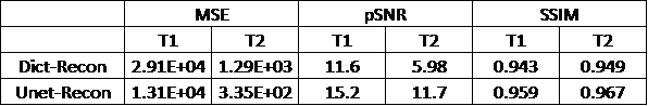
Table 1. Average MSE, pSNR and SSIM for dictionary based reconstructed tissue parameter maps and deep learning predicted tissue parameter maps.