Introduction

The imaging of quantitative MR parameters enables an objective comparison of the investigated tissues on the basis of physical properties and is therefore considered a valuable component of biomarker imaging. Recent work shows that long scan times for qMRI can be reduced to a fraction through data subsampling and model-based reconstructions¹. However, reconstruction with nonlinear models can be time-consuming and thus makes them an ideal candidate for deep learning methods. To the best of our knowledge, there have only been very few approaches of mapping MR parameters by means of deep learning and only one, where a model-augmented neural network is used to estimate M0 and T2 maps². In this work, we propose a neural network that estimates M0 and T1 maps from a corresponding set of subsampled variable flip angle (VFA) images, following the proposed physical model consistency term² that incorporates the signal model into the objective function. We show the acceleration potential on numerical brain phantoms and on retrospectively subsampled in-vivo measurements.

Methods

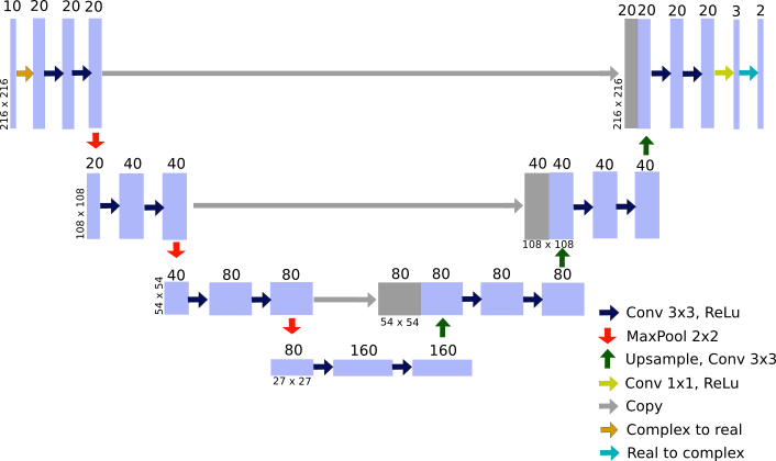
Figure 1 illustrates the implemented U-Net architecture³ which follows a basic encoder-decoder structure. The combination of feature information from the contracting path and spatial information from the expansive path justifies the use of a U-Net for this specific problem, where several input images are mapped to only two parameters maps.
As an input the network receives a set of 10 complex images, separated into real and imaginary channels, from a spoiled gradient echo sequence with flip angles {1°:2°:19°} to cover a wide range of possible T1 values. It’s target is to predict the pseudo proton density M0 and the longitudinal relaxation time T1 by optimizing the network parameters according to:
$$ \theta^* = \arg\min_{\theta} \lambda_{UNet} || UNet(S_{\alpha,u} | \theta) - (M0,T1) ||_2^2 + \lambda_{data} \sum_{\alpha} || F^{-1} P F S_{\alpha} (UNet (S_{\alpha,u} | \theta ))-S_{\alpha,u} ||_2^2$$
The operators $$$F^{-1}$$$ and $$$F$$$ denote the (inverse) Fourier transform, $$$P$$$ is the sampling pattern. The left part is a classic loss term for the forward pass of the neural network whereas the right term ensures signal model fidelity according to the signal equation of a spoiled gradient echo sequence⁴:
$$S_{\alpha}(x) = M0 \frac{\sin(\alpha(x))(1-e^{-TR/T1(x)}) }{1-\cos(\alpha(x))e^{-TR/T1(x)}}$$
The network was trained separately for three different scenarios. A retrospective 1D regular undersampling pattern was equally used for all flip angles with 5% fully-sampled k-space center and additionally sampling every 2^nd, 4^th, or 8^th line, yielding effective acceleration rates of R = 1.89, 3.43, and 5.84.
For training, a generic brain phantom was used, where random Gaussian noise similar to in-vivo noise levels was added. The overall data set consisted of 995 slices which were split into 90% training and 10% test data. The feasibility of this approach was further tested with 420 in-vivo slices from four healthy volunteers by means of transfer-learning which has been shown to be a promising tool for accelerated MRI⁵. Reference parameter maps were generated using iterative model-based reconstruction without spatial regularization¹ and flip angle correction within the signal model was used to compensate for B₁₊ inhomogeneities^6,7.

Results

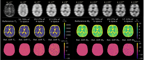
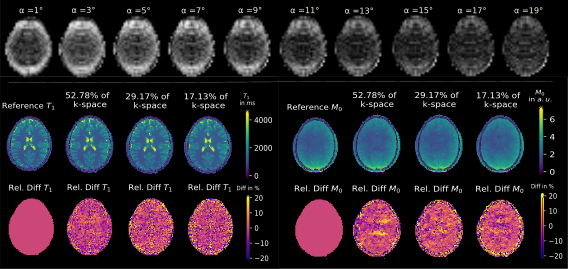
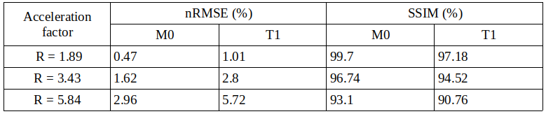
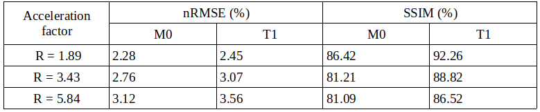
Figure 2 shows exemplary predicted M0 and T1 maps for the subsampled phantom data including an error map denoting the pixel-wise relative error between prediction and reference parameter maps. Table 1 contains the respective normalized root mean squared error (nRMSE) and structural similarity index⁸ (SSIM) for the estimated parameter maps for three different acceleration factors. Figure 3 depicts exemplary parameter maps for subsampled in-vivo data with quantitative results in Table 2.

Discussion

The proposed approach from Liu et al.² is adapted to learn the more complex relation between signal intensity and T1 maps with the signal model term ensuring physical validity. The trained network generates M0 and T1 parameter maps in a time span of only ms which accounts for the huge advantage of using deep learning in image reconstruction provided good training data is available. M0 and T1 maps exhibit excellent visual and quantitative accuracy compared to the fully-sampled reference, also supported by the high similarity of the quantitative metrics given in Table 1. Subsampling with R=5.84 yields predictions with increased pixel-wise outliers. Differences in the estimations for T1 and M0 might be due to the higher complexity of the underlying relation between T1 and the signal intensity and less available information in the training data from a real-valued T1 whereas M0 provides additional phase information. Transferring the learned weights to the in-vivo data yields good results considering the limited amount of training data and even allows to incorporate B₁₊ maps into the signal model. Minor backfolding artifacts are visible in the difference maps which appear less prominent due to noise for increasing acceleration.

Conclusion

We show the feasibility to estimate M0 and T1 maps from a series of highly undersampled VFA images by means of a neural network. Using transfer-learning the network was fine-tuned to work on in-vivo data, demonstrating its clinical potential for future applications even in the case of limited training data. Further research needs to be done on the amount of retrained layers to completely remove backfolding for in-vivo data. Future work could include an extension to multi-coil data and additionally improving B₁₊ inhomogeneity maps in a separate output channel.

Acknowledgements

We gratefully acknowledge the support of NVIDIA Corporation with the donation of the Titan Xp GPU used for this research.