Introduction

Recently, deep learning (DL) based MR reconstruction methods have drown a lot of attentions^1-5. They either learn the algorithm parameters and/or regularization functions by unrolling the optimization algorithms to deep networks, or learn the mapping from aliased images / undersampled k-space data to clean images through a predesigned network. However, the performance of the unrolling-based methods can be further improved by relaxing more constraints. In this work, we take the ISTA-net⁶ as an example to demonstrate how to enhance the performance of an unrolled deep network. Experimental results show that the proposed strategy can achieve superior results from highly undersampled k-space data compared to the initial ISTA-net.

Theory

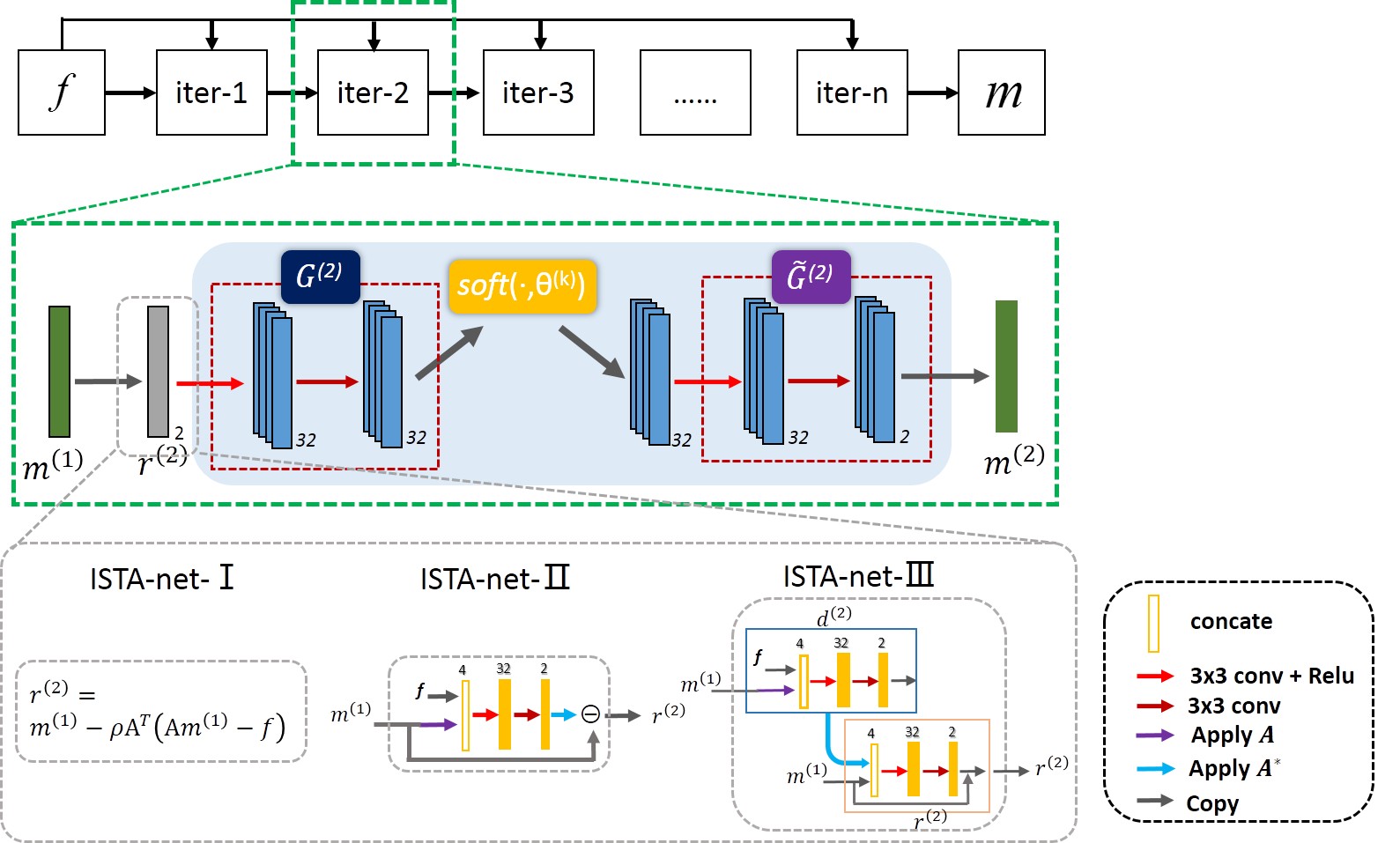
In general, the imaging model of CS-based methods can be written as $$\min_{m}⁡\frac{1}{2} ‖Am-f‖_2^2+λ‖Ψm‖_1 (1)$$ where the first term is the data consistency and the second is the sparse prior. $$$Ψ$$$ is a sparse transform, such as wavelet transform or total variation, $$$m$$$ is the image to be reconstructed, $$$A$$$ is the encoding matrix, $$$f$$$ denotes the acquired k-space data. With the iterative shrinkage-thresholding algorithm (ISTA), problem (1) can be solved with following iterations: $$\begin{cases}r^{(n+1)}=m^{(n)}-ρA^T (Am^{(n)}-f)\\m^{(n+1) }=\min_{m}⁡\frac{1}{2} ‖m-r^{(n+1)}‖_2^2+\tau‖Ψm‖_1\end{cases} (2)$$
ISTA-net-I : learning parameters and transformation
In ISTA-net (here termed as ISTA-net-I), a general nonlinear transform function $$$G$$$ is adopted to sparsify the images, whose parameters are learnable. Therefore, iteration (2) becomes $$\begin{cases}r^{(n+1)}=m^{(n)}-ρA^T (Am^{(n)}-f)\\m^{(n+1) }=\min_{m}⁡\frac{1}{2} ‖G(m)-G(r^{(n+1) )}‖_2^2+\tau‖G(m)‖_1\end{cases} (3)$$ The solution is $$ \begin{cases}r^{(n+1)}=m^{(n)}-ρA^T (Am^{(n)}-f)\\m^{(n+1) }=\widetilde{G}̃(soft(G(r^{(n+1)} ),θ))\end{cases} (4)$$ the step size $$$ρ$$$, shrinkage threshold $$$θ$$$, forward transform $$$G$$$ and the backward transform $$$\widetilde{G}$$$ are the learnable parameters in ISTA-net-I.
ISTA-net-II : learning data consistency
Based on the ISTA-net-I, we further relax the data consistency term $$$‖Am-f‖_2^2$$$ as $$$F(Am,f)$$$, then the deviation of $$$F(Am,f)$$$ can be written as $$$A^T Γ(Am,f)$$$, in which the function $$$Γ$$$ can be accomplished by the deep network. Therefore, the iteration of ISTA-net-II becomes $$ \begin{cases}d^{(n+1)}=Γ(Am^{(n)},f) \\r^{(n+1)}=m^{(n)}-ρA^T d^{(n+1)} \\m^{(n+1) }=\widetilde{G}̃(soft(G(r^{(n+1)} ),θ))\end{cases} (5)$$
ISTA-net-III : learning variable combinations
In ISTA, the residual $$$r^{(n+1)}$$$ is imposed by the difference between the current solution and the deviation of data consistency term, we further use the network to learn the combination of these variables. Thus the solution is as follows: $$ \begin{cases}d^{(n+1)}=Γ(Am^{(n)},f) \\r^{(n+1)}=Λ(m^{(n) },A^T d^{(n+1)}) \\m^{(n+1) }=\widetilde{G}̃(soft(G(r^{(n+1)} ),θ))\end{cases} (6) $$ The operators $$$Γ$$$, $$$Λ$$$, $$$G$$$ and $$$\widetilde{G}̃$$$ are all realized by networks.
ISTA-net-I learns the image transformation through network, whereas ISTA-net-II learns the data consistency additionally, which relaxes the constraint of data fidelity and makes the reconstruction model more general. ISTA-net-III further relax the variable structure constraints based on ISTA-net-II, as the mathematic property such as convergence may not be valid due to the unrolling.

Methods

The structure of ISTA-nets is shown in Fig 1. The convolutions are all 3x3 pixel size, and implemented in TensorFlow using two separate channels representing the real and imaginary parts of MR data.
We trained the network using in-vivo MR datasets. Overall 2100 fully sampled multi-contrast data from 10 subjects with a 3T scanner (MAGNETOM Trio, SIEMENS AG, Erlangen, Germany) were collected and informed consent was obtained from the imaging object in compliance with the IRB policy. The fully sampled data was acquired by a 12-channel head coil with matrix size of 256×256 and adaptively combined to single-channel data and then retrospectively undersampled using Poisson disk sampling mask. 1600 fully sampled data were used to train the networks. We tested the proposed methods on 398 human brain 2D slices, which were acquired from SIEMENS 3T scanner with 32-channel head coil. The data was fully acquired and then manually combined to single-channel and down-sampled for validation. The proposed methods have also been tested on the fully sampled data from another commercial 3T scanners (United Imaging Healthcare, Shanghai, China).

Results

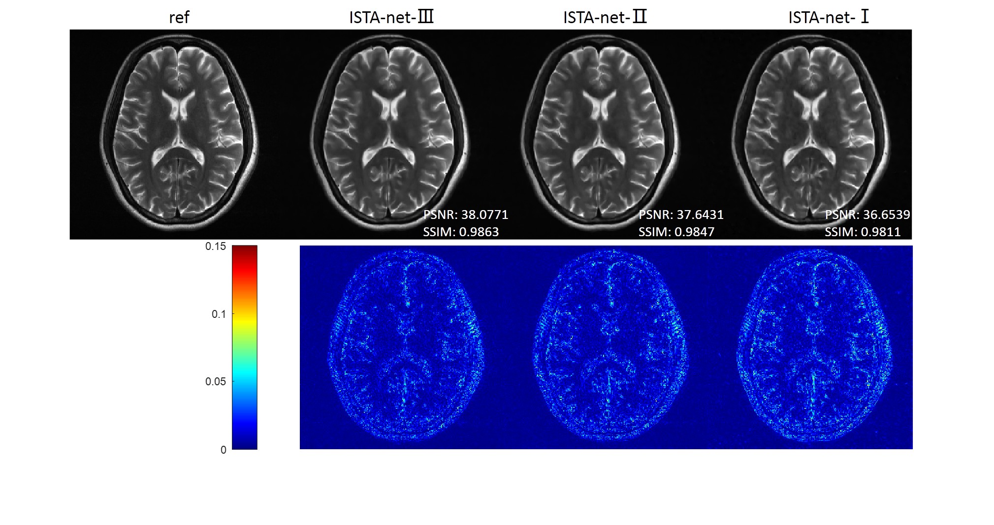
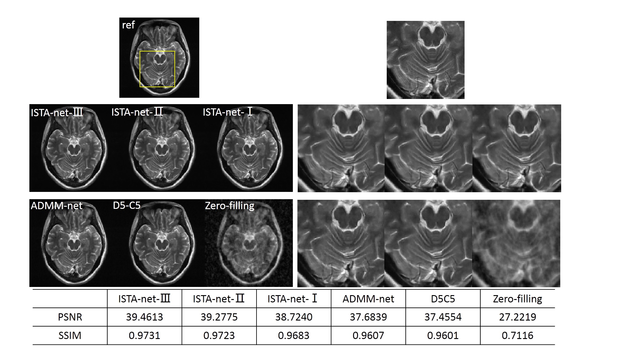
As the constraints in the specific model (1) are gradually relaxed from ISTA-net-I to ISTA-net-III, the reconstruction model becomes more general, and the image quality gradually improves, which is shown in Fig 2.
We also compared the proposed networks with other reconstruction methods: 1) generic-ADMM-CSnet (ADMM-net), an unrolling-based deep learning method learning the regularization function; 2) D5C5, a deep learning method with data consistency; 3) zero-filling, the inverse Fourier transform of undersampled k-space data. The visual comparisons are shown in Fig 3. The zoom-in images of the enclosed part and the corresponding quantitative metrics are also provided.
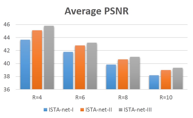
The performance of the proposed strategy on the 398 brain data with different acceleration factors can be seen in Fig 4. The quality of reconstruction deteriorates with larger acceleration factors for each network. Whereas for the fixed acceleration factor, the performance improvement induced by the relaxing can be observed.

Conclusion

In this work, we developed an effective DL-MRI strategy to further integrate classical model-based method and deep network to learn the regularization functions and data consistency simultaneously. The effectiveness of the proposed strategy was validated on the in vivo MR data. The extension to multi-channel MR acquisitions and other applications will be explored in the future.

Acknowledgements

This work was supported in part by the National Natural Science Foundation of China U1805261 and National Key R&D Program of China 2017YFC0108802.