3605
Unsupervised Reconstruction of Continuous Dynamic Radial Acquisitions via CNN-NUFFT Self-Consistency1Radiology, NYU School of Medicine, New York, NY, United States, 2Facebook AI Research, Menlo Park, CA, United States
Synopsis
The introduction of machine learning for medical image reconstruction has opened up new opportunities for reconstruction speed and subsampling; however, acquiring ground truth data is expensive or impossible in the case of dynamic imaging. Here we investigate a technique for optimizing a CNN on continuous radial data by treating the NUFFT-CNN function as an autoencoding deep image prior. Using this method, we are able to reconstruct images that increment over time frames as short as a single spoke. The technique opens up new possibilities for dynamic image reconstruction.
Introduction
The advent of machine learning for medical image reconstruction has facilitated accelerated acquisitions and improved reconstruction times as compared with previous state-of-the-art methods.1,2 A shortcoming of these approaches is the need to acquire fully-sampled ground-truth to train the models in a supervised way. Often, such data is expensive or even impossible to acquire for situations such as dynamic imaging. Here, we investigate a training approach tailored for continuously-acquired radial (GRASP3) data sets that updates network weights via autoencoding in a manner analogous to a deep image prior.4,5Deep image priors are CNNs with structures that intrinsically encode selective image properties.4 Previous work showed that when a randomly-initialized CNN is regressed to an image, it is able to learn useful image features which can serve as regularizers for image reconstruction and modification tasks.4,5 This property could arise from the fact that the architecture of networks such as the U-Net6 are in many ways similar to the wavelet transforms used in compressed sensing. Here we investigate whether CNNs used as a deep image prior can be used to reconstruct continuous radial data. Notably, we employ a CNN sequence autoencoder structure that learns to combine measured spokes with an estimated reconstruction for each time step. The loss is determined by self-consistency between measured spokes and reconstructed spokes extracted from an intermediate NUFFT operator. The approach is flexible and can be applied over arbitrary time scales, offering new opportunities for resolving dynamic contrast curves.
Methods
The model attempts to form a prediction of a set of spokes, $$$y_{t\ in F_c}$$$, given an image buffer, $$$b_c$$$, and a set of spokes, $$$y_{t \in P_c}$$$. Formally,$$\hat{y}_{t \in F_c}=Au_{\theta}(A'Wy_{t \in P_c}, b_c),$$ $$F_c=[t_c-s, ..., t_c+s],$$ $$P_c=[t_c, ..., t_c+v],$$ where $$$F_c$$$ is the set of predicted spoke time points and $$$P_c$$$ is the set of input spoke time points. This is an autoencoder model where the state at $$$t_c$$$ is the reconstructed frame buffer, $$$b_c$$$. To form the predictions, we first pass $$$y_{t \in P_c}$$$ through the density compensation matrix $$$W$$$ and adjoint NUFFT7 operator, $$$A'$$$. Then, we process the adjoint image and the current image estimate, $$$b_c$$$, with a U-Net, $$$u_{\theta}(\cdot)$$$ followed by a forward NUFFT operator, $$$A$$$. This network architecture is shown in Fig. 1. Our goal is to learn the model parameters such that they minimize the error between predicted and measured spokes in the predicted time window, $$$F_c$$$. We accomplish this by minimizing the following cost as a function of $$$\theta$$$:
$$l(\theta) =\sum_{c=1}^D ||\hat{y}_{t \in F_c}-y_{t \in F_c}||_2.$$
We initialized the U-Net with random values and back-propagate through the network at each time step using the ADAM8 optimizer with learning rate 10-3 for 55 epochs. In our experiments we set $$$s$$$ to 34 and $$$v$$$ to 89 and optimized over a total of 1000 time points, incrementing $$$t_c$$$ by 1 during training across the data set (i.e., $$$D$$$=877). We optimized and reconstructed on a single GRASP sequence. For comparison, we also reconstructed with a sliding window method (with 34 spokes per frame and a window step of 10) and using iGRASP3 with 0.03 sparsity parameter, minimizing the iGRASP cost function the split-Bregman optimization algorithm. The iGRASP method used 34 spokes per frame.
Results
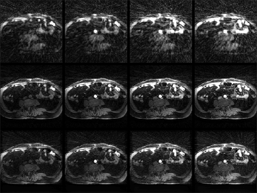
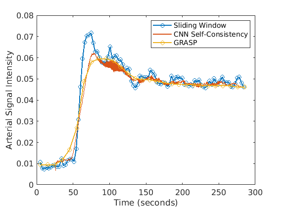
Fig. 2 shows example reconstructions from three methods. The sliding window reconstructions have substantial streaking artifacts that are largely removed with iGRASP reconstruction. The self-consistent CNN method also removes artifacts, but to a lesser extent than iGRASP. Contrast curves from the aorta are shown in Fig. 3, with the sliding window method having the highest (albeit, noisy) temporal fidelity, the self-consistent, CNN method having an intermediate level of temporal fidelity, and the GRASP method having lower temporal fidelity due to its temporal sparsity regularizer.Discussion
Here we demonstrated reconstruction of dynamic MR data with a CNN optimized in an unsupervised manner. The method can reconstruct over any temporal time window - we generated one image for every measured radial spoke after an initial buffer construction with 89 spokes. The unsupervised method substantially reduced aliasing relative to the reference sliding window method, but not to the same extent as GRASP. However, when plotting the aortic contrast time curves, we observed some temporal smoothing of the GRASP method that was less severe with the unsupervised method.We hypothesize that improvements to the proposed methods could be gained by training on multiple data sets. Pre-training the prior could drastically reduce inference time and allow clinically-feasible reconstruction times. Another possible modification is altering the network architecture to better consider long-range dependencies. This could be done by allowing buffers at multiple time points or by incorporating a state space. With such improvements, it may be possible to generate alias-free, single-spoke image updates with a CNN. In the future, we will examine methods for robustly training across different data sets, as well as learning long-term dependencies.
Acknowledgements
We would like to thank NIH grants R01 EB024532 and P41 EB017183.
We would like to thank Tobias Block for useful discussions on iGRASP reconstructions.
* indicates equal contribution to this work.
References
1. Hammernik, K., Klatzer, T., Kobler, E., Recht, M. P., Sodickson, D. K., Pock, T., & Knoll, F. (2018). Learning a variational network for reconstruction of accelerated MRI data. Magnetic resonance in medicine, 79(6), 3055-3071.
2. Schlemper, J., Caballero, J., Hajnal, J. V., Price, A., & Rueckert, D. (2017, June). A deep cascade of convolutional neural networks for MR image reconstruction. In International Conference on Information Processing in Medical Imaging (pp. 647-658). Springer, Cham.
3. Feng, L., Grimm, R., Block, K. T., Chandarana, H., Kim, S., Xu, J., ... & Otazo, R. (2014). Golden‐angle radial sparse parallel MRI: combination of compressed sensing, parallel imaging, and golden‐angle radial sampling for fast and flexible dynamic volumetric MRI. Magnetic resonance in medicine, 72(3), 707-717.
4. Ulyanov, D., Vedaldi, A., & Lempitsky, V. (2018). Deep image prior. In Proceedings of the IEEE Conference on Computer Vision and Pattern Recognition (pp. 9446-9454).
5. Jin, K. H., Gupta, H., Yerly, J., Stuber, M., & Unser, M. (2019). Time-Dependent Deep Image Prior for Dynamic MRI. arXiv preprint arXiv:1910.01684.
6. Ronneberger, O., Fischer, P., & Brox, T. (2015, October). U-net: Convolutional networks for biomedical image segmentation. In International Conference on Medical image computing and computer-assisted intervention (pp. 234-241). Springer, Cham.
7. Fessler, J. A., & Sutton, B. P. (2003). Nonuniform fast Fourier transforms using min-max interpolation. IEEE transactions on signal processing, 51(2), 560-574.
8. Kingma, D. P. & Ba, J. (2014). Adam: A Method for Stochastic Optimization. arxiv:1412.6980
Figures
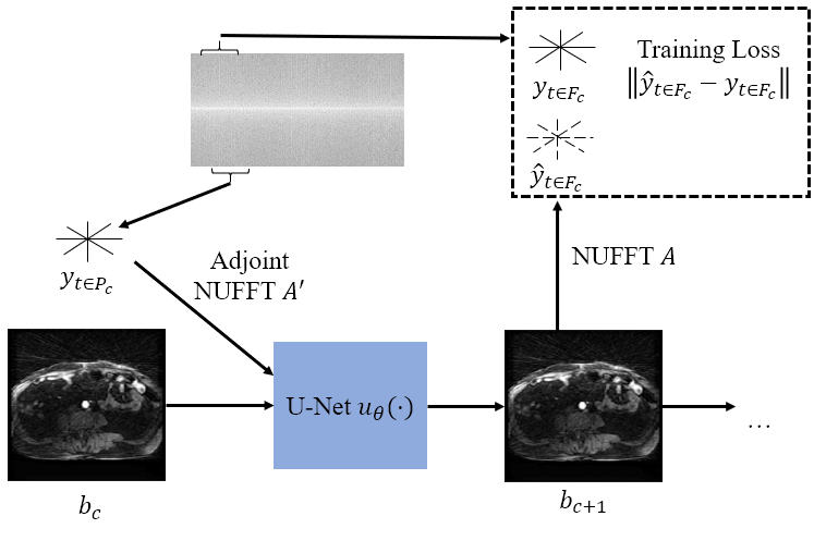
Figure 1: A diagram of the network model. Data within the time window defined by $$$P_c$$$ is passed through an adjoint NUFFT and concatenated with the current buffer, $$$b_c$$$, prior to being passed into a U-Net to produce a new buffer $$$b_{c+1}$$$. A forward NUFFT is applied to $$$b_{c+1}$$$ to produce a prediction, $$$\hat{y}_{t \in F_c}$$$, which is compared to the measured $$$y_{t \in F_c}$$$ to compute the training loss.