Introduction

While impressive image reconstruction performance has been attained recently over a variety of reconstruction tasks using machine learning methods, more robust understanding of these highly-parameterized opaque models is increasingly desired. Recent work such as estimations of uncertainty^1,2 for image reconstructions provide insight towards this direction. In this work, we study the issue of training dataset composition. Although its significant role in the training process is nearly self-evident, the training dataset is typically only qualitatively characterized (e.g. described as collection of modality- and anatomy- specific images). Quantitative characterization of image datasets would enable more systematic study of training dataset composition and their influence on image reconstruction performance. Here we propose to measure the data complexity of training datasets using the Rademacher Complexity metric, and demonstrate its effectiveness in analyzing dataset composition and its effect on neural network training for image reconstruction tasks.

Methods and Results

Intuitively, the Rademacher Complexity^3,4 measures the noise-fitting ability of a class of functions $$$\mathcal{F}$$$ on a domain space Z. In the framework of an image reconstruction task (e.g. supervised learning on a particular neural network architecture), $$$\mathcal{F}$$$ would represent the class of all possible reconstruction functions (as parameterized by all possible weight and bias parameters). Domain space Z would be the raw data domain (e.g. Fourier domain) and a sample $$$S={z_1,...,z_m}$$$ drawn from a distribution D|_z represent the raw data for one m = n x n image in $$$R^{m}$$$ , with $$$f(z_{i})$$$ being the reconstructed pixel values. The Rademacher Complexity is defined as $$ R_{m}(\mathcal{F})=\mathrm{E}_{D}\left[\mathrm{E}_{\sigma}\left[\sup _{f \in \mathcal{F}}\left(\frac{1}{m} \sum_{i=1}^{m} \sigma_{i} f\left(z_{i}\right)\right)\right]\right ]$$
where Rademacher variables σ_i,...,σ_m are independent random variables uniformly chosen from {-1,+1} and can be interpreted as a binary noise image. More generally, we can study the Rademacher Complexity of hypothesis-class or image-domain data, on sets $$$A \subseteq R^{m}$$$, with $$ R_{m}(\mathcal{A})=\mathrm{E}_{\sigma}\left[\sup _{a \in \mathcal{A}}\left(\frac{1}{m} \sum_{i=1}^{m} \sigma_{i} a_i\right)\right] $$ in order to quantify the data complexity of training set images.

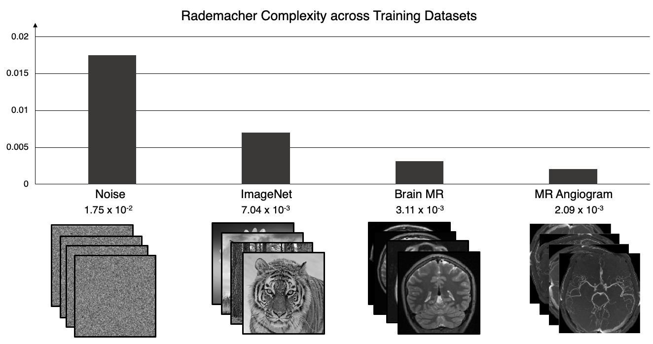
We measure the approximate Rademacher Complexity of four domains of image data at 128 x 128 matrix size: white Gaussian noise, generic photographs from ImageNet⁵, T₁-weighted brain MR magnitude images⁶, and maximum intensity projected (MIP) MR angiogram magnitudes⁷. To compute this measure for each dataset, we used 10,000 randomly generated Rademacher variable binary noise images and 10,000 image samples from each dataset.

As shown in Figure 1, the computed Rademacher Complexity is 1.75x10^-2 for white Gaussian noise, 7.04 x10^-3 for ImageNet, 3.11 x10^-3 for T₁ brain MR, and 2.09 x 10^-3 for MRA; this quantitative decrease from noise to MRA images corresponds with a visually perceptible decrease in spatial complexity.
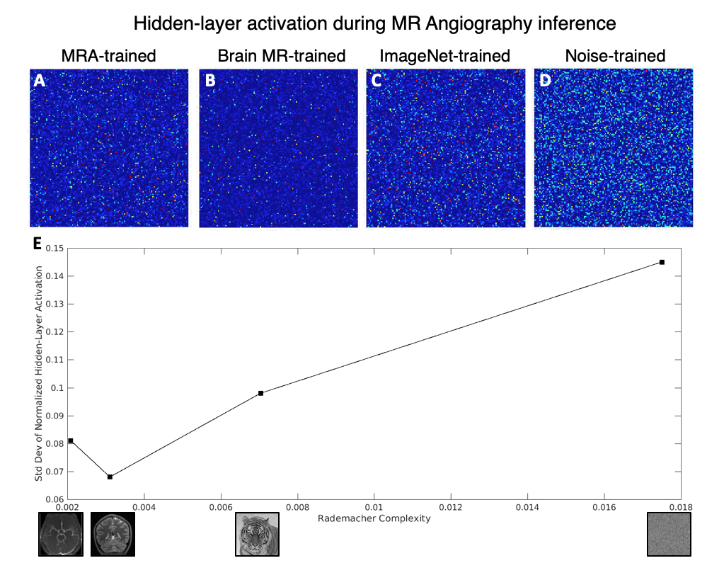
Because dataset composition is a critical component in the training process of neural network reconstruction models, we investigated how this variation in Rademacher Complexity of the datasets coincides with neural network activity in differently-trained models. Here we used a variation of the AUTOMAP⁸ neural network architecture and using canonical cartesian Fourier-domain raw data, but similar experiments can be performed on various reconstruction networks and various raw data domains. In order to isolate the domain-transform aspect of the reconstruction process in this work, we removed the influence of convolutional processing and only retained the two fully-connected layers of the network. The datasets described above were phase-modulated with low-spatial-frequency sinusoids⁸ in order to train the network to properly reconstruct both magnitude and phase information, and then 2D Fourier transformed to form the input to the network for training, for all four datasets. (more details of the training protocol can be found in reference⁸ )

When performing inference on test data with the variously trained networks, we observe that for both low-complexity brain and vasculature data, the hidden-layer node activity of the fully-connected network generally increases with Rademacher complexity. (Fig 2) Surprisingly, when reconstructing angiogram images, the most efficient representation is generated by the brain-MR-trained model (2B), suggesting that there may be a non-monotonic, optimal “middle” range of data complexity for training reconstruction networks, even if the test data is low in complexity. The standard deviation of the hidden-layer activations, a summary statistic of the strength of the activations (which have mean near zero), is plotted against the Rademacher Complexity of the trained networks.

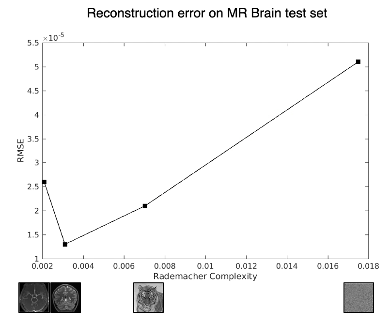
We finally show root mean squared error (RMSE) on the reconstructions for a T₁-weighted brain test set when reconstructed with the differently trained networks in Figure 3. While it is expected that the brain-trained network would perform the best, here we relate the reconstructions to the Rademacher Complexities, and observe a rudimentary “smoothness” whereby the ImageNet-trained network trained on data with complexity between noise and brain images achieves reconstruction performance correspondingly. This suggests that we may be able to predict reconstruction performance before even training a dataset by comparing the Rademacher Complexities between the training and test sets. As Rademacher Complexities (and similar metrics) are further explored, we can begin to craft training datasets to optimize reconstruction performance with more principled and quantitative approaches.

Acknowledgements

No acknowledgement found.